More about forecasting in cienciadedatos.net
- ARIMA and SARIMAX models with python
- Time series forecasting with machine learning
- Forecasting time series with gradient boosting: XGBoost, LightGBM and CatBoost
- Forecasting time series with XGBoost
- Global Forecasting Models: Multi-series forecasting
- Global Forecasting Models: Comparative Analysis of Single and Multi-Series Forecasting Modeling
- Probabilistic forecasting
- Forecasting with deep learning
- Forecasting energy demand with machine learning
- Forecasting web traffic with machine learning
- Intermittent demand forecasting
- Modelling time series trend with tree-based models
- Bitcoin price prediction with Python
- Stacking ensemble of machine learning models to improve forecasting
- Interpretable forecasting models
- Mitigating the Impact of Covid on Forecasting Models
- Forecasting time series with missing values

Introduction
A time series is a succession of chronologically ordered data spaced at equal or unequal intervals. The forecasting process consists of predicting the future value of a time series, either by modeling the series solely based on its past behavior (autoregressive) or by using other external variables.
This guide explores the use of scikit-learn regression models for time series forecasting. Specifically, it introduces skforecast, an intuitive library equipped with essential classes and functions to customize any Scikit-learn regression model to effectively address forecasting challenges.
✏️ Note
This document serves as an introductory guide to machine learning based forecasting using skforecast. For more advanced and detailed examples, please explore:
These resources delve deeper into diverse applications, offering insights and practical demonstrations of advanced techniques in time series forecasting using machine learning methodologies.Machine learning for forecasting
In order to apply machine learning models to forecasting problems, the time series must be transformed into a matrix in which each value is related to the time window (lags) that precedes it.
In a time series context, a lag with respect to a time step $t$ is defined as the values of the series at previous time steps. For example, lag 1 is the value at time step $t − 1$ and lag $m$ is the value at time step $t − m$.
![]()
This type of transformation also allows to include additional variables.
![]()
Once the data are rearranged into the new shape, any regression model can be trained to predict the next value (step) of the series. During model training, every row is considered a separate data instance, where values at lags 1, 2, ... $p$ are considered predictors for the target quantity of the time series at time step $t + 1$.
Multi-Step Time Series Forecasting
When working with time series, it is seldom needed to predict only the next element in the series ($t_{+1}$). Instead, the most common goal is to predict a whole future interval (($t_{+1}$), ..., ($t_{+n}$)) or a far point in time ($t_{+n}$). Several strategies allow generating this type of prediction.
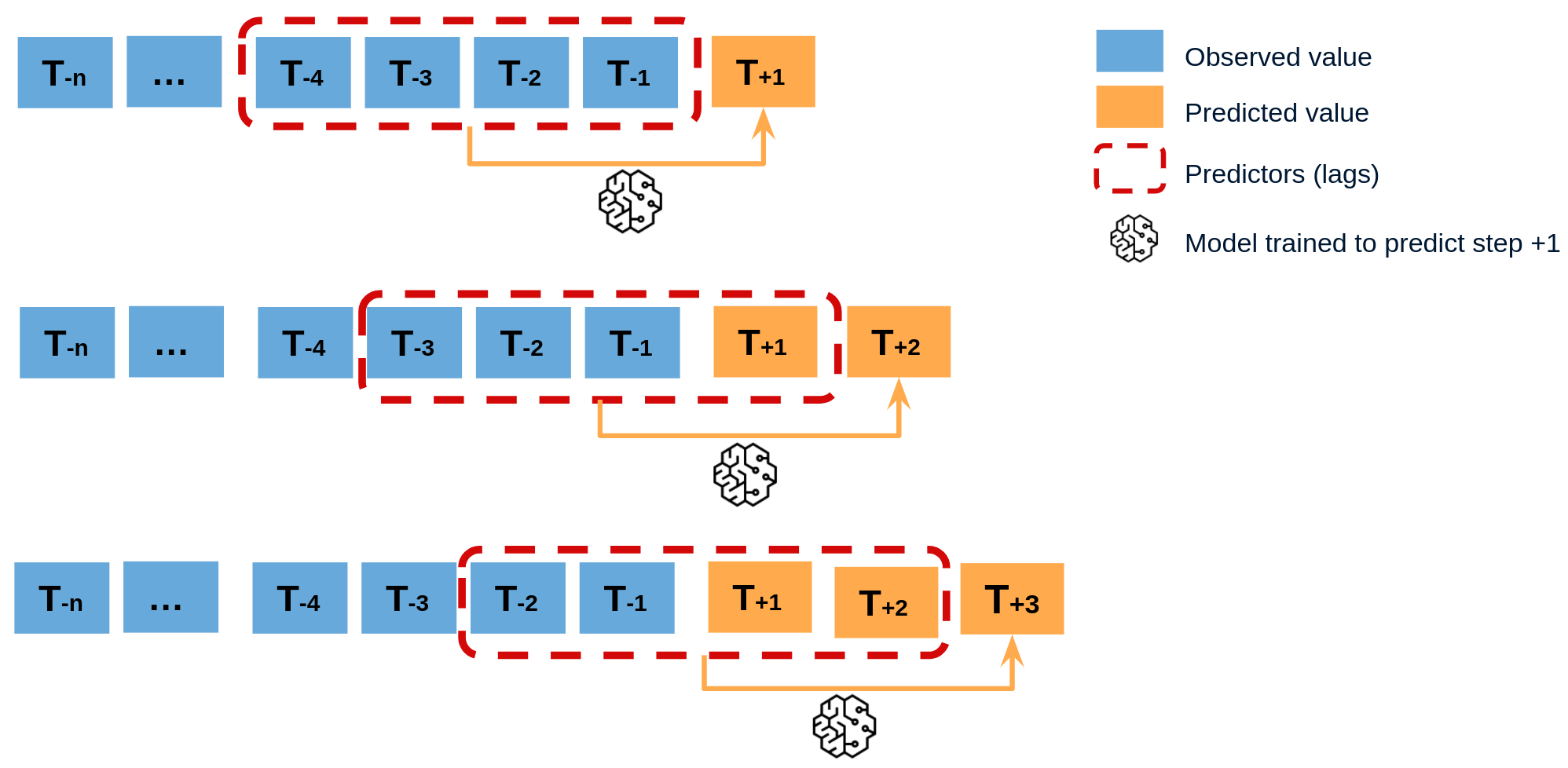
Recursive multi-step forecasting
Since the value $t_{n-1}$ is required to predict $t_{n}$, and $t_{n-1}$ is unknown, a recursive process is applied in which, each new prediction, is based on the previous one. This process is known as recursive forecasting or recursive multi-step forecasting and can be easily generated with the ForecasterRecursive class.

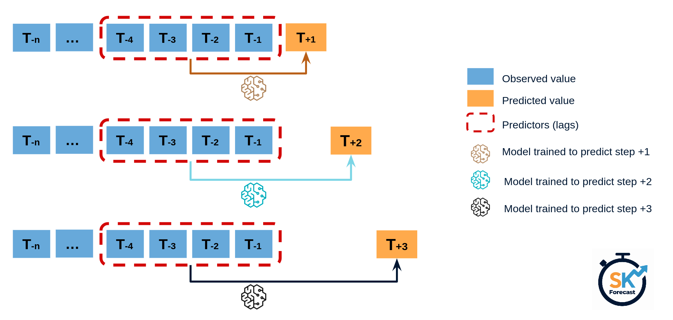
Direct multi-step forecasting
Direct multi-step forecasting consists of training a different model for each step of the forecast horizon. For example, to predict the next 5 values of a time series, 5 different models are trained, one for each step. As a result, the predictions are independent of each other.

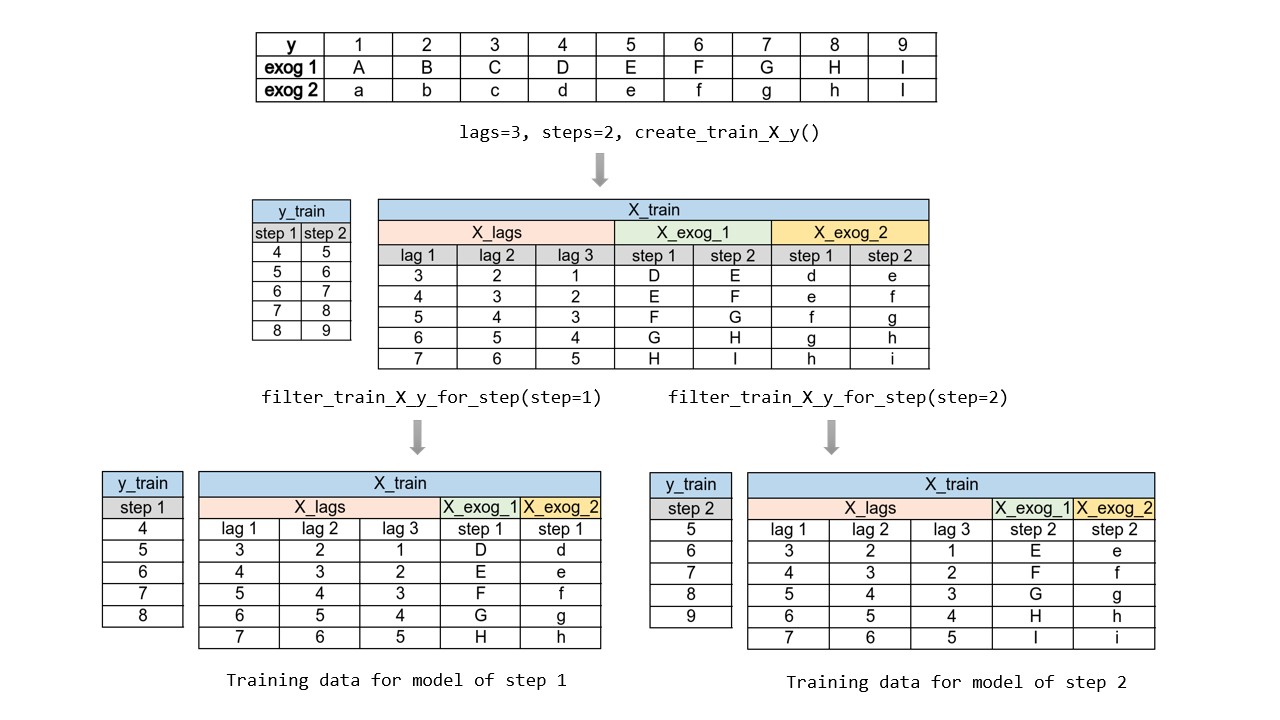
The main complexity of this approach is to generate the correct training matrices for each model. The ForecasterDirect class of the skforecast library automates this process. It is also important to bear in mind that this strategy has a higher computational cost since it requires the train of multiple models. The following diagram shows the process for a case in which the response variable and two exogenous variables are available.
Forecasting multi-output
Some machine learning models, such as long short-term memory (LSTM) neural networks, can predict multiple values of a sequence simultaneously (one-shot). This strategy implemented in the ForecasterRnn class of the skforecast library
Libraries
The libraries used in this document are:
# Data manipulation
# ==============================================================================
import numpy as np
import pandas as pd
from skforecast.datasets import fetch_dataset
# Plots
# ==============================================================================
import matplotlib.pyplot as plt
from skforecast.plot import set_dark_theme
# Modeling and Forecasting
# ==============================================================================
import sklearn
from sklearn.linear_model import Ridge
from sklearn.ensemble import RandomForestRegressor
from sklearn.metrics import mean_squared_error, mean_absolute_error
from sklearn.preprocessing import StandardScaler
import skforecast
from skforecast.recursive import ForecasterRecursive
from skforecast.direct import ForecasterDirect
from skforecast.model_selection import TimeSeriesFold, grid_search_forecaster, backtesting_forecaster
from skforecast.preprocessing import RollingFeatures
from skforecast.utils import save_forecaster, load_forecaster
from skforecast.metrics import calculate_coverage
from skforecast.plot import plot_prediction_intervals
import shap
# Warnings configuration
# ==============================================================================
import warnings
warnings.filterwarnings('once')
color = '\033[1m\033[38;5;208m'
print(f"{color}Version skforecast: {skforecast.__version__}")
print(f"{color}Version scikit-learn: {sklearn.__version__}")
print(f"{color}Version pandas: {pd.__version__}")
print(f"{color}Version numpy: {np.__version__}")
Version skforecast: 0.22.0 Version scikit-learn: 1.7.2 Version pandas: 2.3.3 Version numpy: 2.1.3
Data
A time series is available with the monthly expenditure (millions of dollars) on corticosteroid drugs that the Australian health system had between 1991 and 2008. It is intended to create an autoregressive model capable of predicting future monthly expenditures. The data used in the examples of this document have been obtained from the magnificent book Forecasting: Principles and Practice by Rob J Hyndman and George Athanasopoulos.
# Data download
# ==============================================================================
data = fetch_dataset(name='h2o_exog', raw=True)
╭─────────────────────────────────── h2o_exog ────────────────────────────────────╮ │ Description: │ │ Monthly expenditure ($AUD) on corticosteroid drugs that the Australian health │ │ system had between 1991 and 2008. Two additional variables (exog_1, exog_2) are │ │ simulated. │ │ │ │ Source: │ │ Hyndman R (2023). fpp3: Data for Forecasting: Principles and Practice (3rd │ │ Edition). http://pkg.robjhyndman.com/fpp3package/, │ │ https://github.com/robjhyndman/fpp3package, http://OTexts.com/fpp3. │ │ │ │ URL: │ │ https://raw.githubusercontent.com/skforecast/skforecast- │ │ datasets/main/data/h2o_exog.csv │ │ │ │ Shape: 195 rows x 4 columns │ ╰─────────────────────────────────────────────────────────────────────────────────╯
The column date has been stored as a string. To convert it to datetime the pd.to_datetime() function can be use. Once in datetime format, and to make use of Pandas functionalities, it is set as an index. Also, since the data is monthly, the frequency is set as Monthly Started 'MS'.
# Data preparation
# ==============================================================================
data = data.rename(columns={'fecha': 'date'})
data['date'] = pd.to_datetime(data['date'], format='%Y-%m-%d')
data = data.set_index('date')
data = data.asfreq('MS')
data = data.sort_index()
data.head()
| y | exog_1 | exog_2 | |
|---|---|---|---|
| date | |||
| 1992-04-01 | 0.379808 | 0.958792 | 1.166029 |
| 1992-05-01 | 0.361801 | 0.951993 | 1.117859 |
| 1992-06-01 | 0.410534 | 0.952955 | 1.067942 |
| 1992-07-01 | 0.483389 | 0.958078 | 1.097376 |
| 1992-08-01 | 0.475463 | 0.956370 | 1.122199 |
When using the asfreq() method in Pandas, any gaps in the time series will be filled with NaN values to match the specified frequency. Therefore, it is essential to check for any missing values that may occur after this transformation.
# Missing values
# ==============================================================================
print(f'Number of rows with missing values: {data.isnull().any(axis=1).sum()}')
Number of rows with missing values: 0
Although it is unnecessary, since a frequency has been established, it is possible to verify that the time series is complete.
# Verify that the time index is complete
# ==============================================================================
start_date = data.index.min()
end_date = data.index.max()
complete_date_range = pd.date_range(start=start_date, end=end_date, freq=data.index.freq)
is_index_complete = (data.index == complete_date_range).all()
print(f"Index complete: {is_index_complete}")
Index complete: True
# Fill gaps in the time index
# ==============================================================================
# data.asfreq(freq='30min', fill_value=np.nan)
The last 36 months are used as the test set to evaluate the predictive capacity of the model.
# Split data into train-test
# ==============================================================================
steps = 36
data_train = data[:-steps]
data_test = data[-steps:]
print(
f"Train dates : {data_train.index.min()} --- "
f"{data_train.index.max()} (n={len(data_train)})"
)
print(
f"Test dates : {data_test.index.min()} --- "
f"{data_test.index.max()} (n={len(data_test)})"
)
set_dark_theme()
fig, ax = plt.subplots(figsize=(6, 2.5))
data_train['y'].plot(ax=ax, label='train')
data_test['y'].plot(ax=ax, label='test')
ax.legend();
Train dates : 1992-04-01 00:00:00 --- 2005-06-01 00:00:00 (n=159) Test dates : 2005-07-01 00:00:00 --- 2008-06-01 00:00:00 (n=36)

Recursive multi-step forecasting
With the ForecasterRecursive class, a forecasting model is created and trained using a RandomForestRegressor estimator with a time window of 6 lags. This means that the model uses the previous 6 months as predictors. Six lags are used as a starting point; the optimal number will be determined during hyperparameter tuning.
# Create and train forecaster
# ==============================================================================
forecaster = ForecasterRecursive(
estimator = RandomForestRegressor(random_state=123),
lags = 6
)
forecaster.fit(y=data_train['y'])
forecaster
ForecasterRecursive
General Information
- Estimator: RandomForestRegressor
- Lags: [1 2 3 4 5 6]
- Window features: None
- Window size: 6
- Series name: y
- Exogenous included: False
- Categorical features: auto
- Weight function included: False
- Differentiation order: None
- Drop NaN from series: False
- Creation date: 2026-04-23 11:40:50
- Last fit date: 2026-04-23 11:40:50
- Skforecast version: 0.22.0
- Python version: 3.13.12
- Forecaster id: None
Exogenous Variables
None
Data Transformations
- Transformer for y: None
- Transformer for exog: None
Training Information
- Training range: [Timestamp('1992-04-01 00:00:00'), Timestamp('2005-06-01 00:00:00')]
- Training index type: DatetimeIndex
- Training index frequency:
Estimator Parameters
-
{'bootstrap': True, 'ccp_alpha': 0.0, 'criterion': 'squared_error', 'max_depth': None, 'max_features': 1.0, 'max_leaf_nodes': None, 'max_samples': None, 'min_impurity_decrease': 0.0, 'min_samples_leaf': 1, 'min_samples_split': 2, 'min_weight_fraction_leaf': 0.0, 'monotonic_cst': None, 'n_estimators': 100, 'n_jobs': None, 'oob_score': False, 'random_state': 123, 'verbose': 0, 'warm_start': False}
Fit Kwargs
-
{}
Prediction
Once the model is trained, the test data is predicted (36 months into the future).
# Predictions
# ==============================================================================
steps = 36
predictions = forecaster.predict(steps=steps)
predictions.head(5)
2005-07-01 0.878756 2005-08-01 0.882167 2005-09-01 0.973184 2005-10-01 0.983678 2005-11-01 0.849494 Freq: MS, Name: pred, dtype: float64
# Plot predictions versus test data
# ==============================================================================
fig, ax = plt.subplots(figsize=(6, 2.5))
data_train['y'].plot(ax=ax, label='train')
data_test['y'].plot(ax=ax, label='test')
predictions.plot(ax=ax, label='predictions')
ax.legend();

Forecasting error in the test set
To quantify the error the model makes in its predictions, the mean squared error (mse) metric is used.
# Test error
# ==============================================================================
error_mse = mean_squared_error(
y_true = data_test['y'],
y_pred = predictions
)
print(f"Test error (MSE): {error_mse}")
Test error (MSE): 0.0732683397612037
Hyperparameter tuning
The trained ForecasterRecursive uses a 6 lags as predictors and a Random Forest model with the default hyperparameters. However, there is no reason why these values are the most suitable. Skforecast provide several search strategies to find the best combination of hyperparameters and lags. In this case, the grid_search_forecaster function is used. It compares the results obtained with each combinations of hyperparameters and lags, and identify the best one.
💡 Tip
The computational cost of hyperparameter tuning depends heavily on the backtesting approach chosen to evaluate each hyperparameter combination. In general, the duration of the tuning process increases with the number of re-trains involved in the backtesting.
To effectively speed up the prototyping phase, it is highly recommended to adopt a two-step strategy. First, use refit=False during the initial search to narrow down the range of values. Then, focus on the identified region of interest and apply a tailored backtesting strategy that meets the specific requirements of the use case. For more tips on backtesting strategies, see Hyperparameter tuning and lags selection.
# Hyperparameters: grid search
# ==============================================================================
forecaster = ForecasterRecursive(
estimator = RandomForestRegressor(random_state=123),
lags = 12 # This value will be replaced in the grid search
)
# Training and validation folds
cv = TimeSeriesFold(
steps = 36,
initial_train_size = int(len(data_train) * 0.5),
refit = False,
fixed_train_size = False,
)
# Candidate values for lags
lags_grid = [10, 20]
# Candidate values for estimator's hyperparameters
param_grid = {
'n_estimators': [100, 250],
'max_depth': [3, 8]
}
results_grid = grid_search_forecaster(
forecaster = forecaster,
y = data_train['y'],
cv = cv,
param_grid = param_grid,
lags_grid = lags_grid,
metric = 'mean_squared_error',
return_best = True,
n_jobs = 'auto',
verbose = False
)
# Search results
# ==============================================================================
results_grid
| lags | lags_label | params | mean_squared_error | max_depth | n_estimators | |
|---|---|---|---|---|---|---|
| 0 | [1, 2, 3, 4, 5, 6, 7, 8, 9, 10, 11, 12, 13, 14... | [1, 2, 3, 4, 5, 6, 7, 8, 9, 10, 11, 12, 13, 14... | {'max_depth': 3, 'n_estimators': 250} | 0.021773 | 3 | 250 |
| 1 | [1, 2, 3, 4, 5, 6, 7, 8, 9, 10, 11, 12, 13, 14... | [1, 2, 3, 4, 5, 6, 7, 8, 9, 10, 11, 12, 13, 14... | {'max_depth': 8, 'n_estimators': 250} | 0.022068 | 8 | 250 |
| 2 | [1, 2, 3, 4, 5, 6, 7, 8, 9, 10, 11, 12, 13, 14... | [1, 2, 3, 4, 5, 6, 7, 8, 9, 10, 11, 12, 13, 14... | {'max_depth': 3, 'n_estimators': 100} | 0.022569 | 3 | 100 |
| 3 | [1, 2, 3, 4, 5, 6, 7, 8, 9, 10, 11, 12, 13, 14... | [1, 2, 3, 4, 5, 6, 7, 8, 9, 10, 11, 12, 13, 14... | {'max_depth': 8, 'n_estimators': 100} | 0.023562 | 8 | 100 |
| 4 | [1, 2, 3, 4, 5, 6, 7, 8, 9, 10] | [1, 2, 3, 4, 5, 6, 7, 8, 9, 10] | {'max_depth': 3, 'n_estimators': 100} | 0.063144 | 3 | 100 |
| 5 | [1, 2, 3, 4, 5, 6, 7, 8, 9, 10] | [1, 2, 3, 4, 5, 6, 7, 8, 9, 10] | {'max_depth': 3, 'n_estimators': 250} | 0.064241 | 3 | 250 |
| 6 | [1, 2, 3, 4, 5, 6, 7, 8, 9, 10] | [1, 2, 3, 4, 5, 6, 7, 8, 9, 10] | {'max_depth': 8, 'n_estimators': 250} | 0.064546 | 8 | 250 |
| 7 | [1, 2, 3, 4, 5, 6, 7, 8, 9, 10] | [1, 2, 3, 4, 5, 6, 7, 8, 9, 10] | {'max_depth': 8, 'n_estimators': 100} | 0.068730 | 8 | 100 |
The best results are obtained using a time window of 20 lags and a Random Forest set up of {'max_depth': 3, 'n_estimators': 250}.
Final model
Finally, a ForecasterRecursive is trained with the optimal configuration found. This step is not necessary if return_bestis set to True in the grid_search_forecaster function.
# Create and train forecaster with the best hyperparameters and lags found
# ==============================================================================
estimator = RandomForestRegressor(n_estimators=250, max_depth=3, random_state=123)
forecaster = ForecasterRecursive(
estimator = estimator,
lags = 20
)
forecaster.fit(y=data_train['y'])
# Predictions
# ==============================================================================
predictions = forecaster.predict(steps=steps)
# Plot predictions versus test data
# ==============================================================================
fig, ax = plt.subplots(figsize=(6, 2.5))
data_train['y'].plot(ax=ax, label='train')
data_test['y'].plot(ax=ax, label='test')
predictions.plot(ax=ax, label='predictions')
ax.legend();

# Test error
# ==============================================================================
error_mse = mean_squared_error(
y_true = data_test['y'],
y_pred = predictions
)
print(f"Test error (MSE): {error_mse}")
Test error (MSE): 0.004356831371529948
The optimal combination of hyperparameters significantly reduces test error.
Backtesting
To obtain a robust estimate of the model's predictive capacity, a backtesting process is carried out. The process of backtesting consists of evaluating the performance of a predictive model by applying it retrospectively to historical data. Therefore, it is a special type of cross-validation applied to the previous period(s).
✏️ Note
To ensure an accurate evaluation of your model and gain confidence in its predictive performance on new data, it is critical to employ an appropriate backtesting strategy. Factors such as use case characteristics, available computing resources and time intervals between predictions need to be considered to determine which strategy to use.
In general, the more closely the backtesting process resembles the actual scenario in which the model is used, the more reliable the estimated metric will be. For more information about backtesting, visit Which strategy should I use?.
Backtesting with refit and increasing training size (fixed origin)
The model is trained each time before making predictions. With this configuration, the model uses all the data available so far. It is a variation of the standard cross-validation but, instead of making a random distribution of the observations, the training set increases sequentially, maintaining the temporal order of the data.
Backtesting with refit and fixed training size (rolling origin)
A technique similar to the previous one but, in this case, the forecast origin rolls forward, therefore, the size of training remains constant. This is also known as time series cross-validation or walk-forward validation.
Backtesting with intermittent refit
The model is retrained every $n$ iterations of predictions.
💡 Tip
This strategy usually achieves a good balance between the computational cost of retraining and avoiding model degradation.
Backtesting without refit
After an initial train, the model is used sequentially without updating it and following the temporal order of the data. This strategy has the advantage of being much faster since the model is trained only once. However, the model does not incorporate the latest data available, so it may lose predictive capacity over time.
Backtesting con with stride
This method involves controlling how far the test set moves forward between folds. For example, you might want to forecast the next 30 days but generate a new forecast every 7 days. In this setup, each test window is 30 days long (steps=30), while the stride between folds is one week (fold_stride=7). This means forecasts overlap, and the same observations are predicted multiple times, which provides a richer view of model consistency and stability across different forecast origins.
Depending on the relation between steps and fold_stride, the output may include repeated indexes (if fold_stride < steps) or gaps (if fold_stride > steps).
Skip folds
All of the above backtesting strategies can be combined with the option to skip a certain number of folds by setting the skip_folds argument. Since the model predicts fewer points in time, the computational cost is reduced and the backtesting process is faster. This is particularly useful when one is interested in an approximate estimate of the model's performance, but does not require an exact evaluation, for example, when searching for hyperparameters. If skip_folds is an integer, every 'skip_folds'-th is returned. If skip_folds is a list, the folds in the list are skipped. For example, if skip_folds = 3, and there are 10 folds, the returned folds will be [0, 3, 6, 9]. If skip_folds is a list [1, 2, 3], the returned folds will be [0, 4, 5, 6, 7, 8, 9].
Skforecast library has multiple backtesting strategies implemented. Regardless of which one is used, it is important not to include test data in the search process to avoid overfitting problems.
For this example, a Backtesting with Refit and Increasing Training Size (Fixed Origin) strategy is followed. Internally, the process that the function applies is:
In the first iteration, the model is trained with the observations selected for the initial training (in this case, 87). Then, the next 36 observations are predicted.
In the second iteration, the model is retrained by adding 36 observations to the initial training set (87 + 36), and then the next 36 observations are predicted.
This process is repeated until all available observations are used. Following this strategy, the training set increases in each iteration with as many observations as steps are being predicted.
The TimeSeriesFold class is designed to generate the partitions used in the backtesting process to train and evaluate the model. By leveraging its various arguments, it provides extensive flexibility, enabling the simulation of scenarios such as refit, no refit, rolling origin, and others. The split method returns the index positions of the time series corresponding to each partition. When as_pandas=True is specified, the output is a DataFrame with detailed information, including descriptive column names.
# Backtesting partitions using TimeSeriesFold
# ==============================================================================
cv = TimeSeriesFold(
steps = 12 * 3,
initial_train_size = len(data) - 12 * 9, # Last 9 years are separated for the backtest
window_size = 20,
fixed_train_size = False,
refit = True,
)
cv.split(X=data, as_pandas=True)
Information of folds
--------------------
Number of observations used for initial training: 87
Number of observations used for backtesting: 108
Number of folds: 3
Number skipped folds: 0
Number of steps per fold: 36
Number of steps to exclude between last observed data (last window) and predictions (gap): 0
Fold: 0
Training: 1992-04-01 00:00:00 -- 1999-06-01 00:00:00 (n=87)
Validation: 1999-07-01 00:00:00 -- 2002-06-01 00:00:00 (n=36)
Fold: 1
Training: 1992-04-01 00:00:00 -- 2002-06-01 00:00:00 (n=123)
Validation: 2002-07-01 00:00:00 -- 2005-06-01 00:00:00 (n=36)
Fold: 2
Training: 1992-04-01 00:00:00 -- 2005-06-01 00:00:00 (n=159)
Validation: 2005-07-01 00:00:00 -- 2008-06-01 00:00:00 (n=36)
| fold | train_start | train_end | last_window_start | last_window_end | test_start | test_end | test_start_with_gap | test_end_with_gap | fit_forecaster | |
|---|---|---|---|---|---|---|---|---|---|---|
| 0 | 0 | 0 | 87 | 67 | 87 | 87 | 123 | 87 | 123 | True |
| 1 | 1 | 0 | 123 | 103 | 123 | 123 | 159 | 123 | 159 | True |
| 2 | 2 | 0 | 159 | 139 | 159 | 159 | 195 | 159 | 195 | True |
When used in combination with backtesting_forecaster, the window_size argument does not need to be specified. This is because backtesting_forecaster automatically sets this value based on the forecaster's configuration. This ensures that the backtesting process is perfectly aligned with the forecaster's requirements.
# Backtesting
# ==============================================================================
cv = TimeSeriesFold(
steps = 12 * 3,
initial_train_size = len(data) - 12 * 9,
fixed_train_size = False,
refit = True,
)
metric, predictions_backtest = backtesting_forecaster(
forecaster = forecaster,
y = data['y'],
cv = cv,
metric = 'mean_squared_error',
verbose = True
)
metric
Information of folds
--------------------
Number of observations used for initial training: 87
Number of observations used for backtesting: 108
Number of folds: 3
Number skipped folds: 0
Number of steps per fold: 36
Number of steps to exclude between last observed data (last window) and predictions (gap): 0
Fold: 0
Training: 1992-04-01 00:00:00 -- 1999-06-01 00:00:00 (n=87)
Validation: 1999-07-01 00:00:00 -- 2002-06-01 00:00:00 (n=36)
Fold: 1
Training: 1992-04-01 00:00:00 -- 2002-06-01 00:00:00 (n=123)
Validation: 2002-07-01 00:00:00 -- 2005-06-01 00:00:00 (n=36)
Fold: 2
Training: 1992-04-01 00:00:00 -- 2005-06-01 00:00:00 (n=159)
Validation: 2005-07-01 00:00:00 -- 2008-06-01 00:00:00 (n=36)
| mean_squared_error | |
|---|---|
| 0 | 0.010233 |
# Plot backtest predictions vs real values
# ==============================================================================
fig, ax = plt.subplots(figsize=(6, 2.5))
data.loc[predictions_backtest.index, 'y'].plot(ax=ax, label='test')
predictions_backtest['pred'].plot(ax=ax, label='predictions')
ax.legend();

Model explanaibility (Feature importance)
Due to the complex nature of many modern machine learning models, such as ensemble methods, they often function as black boxes, making it difficult to understand why a particular prediction was made. Explanability techniques aim to demystify these models, providing insight into their inner workings and helping to build trust, improve transparency, and meet regulatory requirements in various domains. Enhancing model explainability not only helps to understand model behavior, but also helps to identify biases, improve model performance, and enable stakeholders to make more informed decisions based on machine learning insights.
Skforecast is compatible with some of the most popular model explainability methods: model-specific feature importances, SHAP values, and partial dependence plots.
Model-specific feature importance
# Extract feature importance
# ==============================================================================
importance = forecaster.get_feature_importances()
importance.head(10)
| feature | importance | |
|---|---|---|
| 11 | lag_12 | 0.815564 |
| 1 | lag_2 | 0.086286 |
| 13 | lag_14 | 0.019047 |
| 9 | lag_10 | 0.013819 |
| 2 | lag_3 | 0.012943 |
| 14 | lag_15 | 0.009637 |
| 0 | lag_1 | 0.009141 |
| 10 | lag_11 | 0.008130 |
| 7 | lag_8 | 0.007377 |
| 8 | lag_9 | 0.005268 |
⚠️ Warning
The get_feature_importances() method will only return values if the forecaster's estimator has either the coef_ or feature_importances_ attribute, which is the default in scikit-learn.
Shap values
SHAP (SHapley Additive exPlanations) values are a popular method for explaining machine learning models, as they help to understand how variables and values influence predictions visually and quantitatively.
It is possible to generate SHAP-values explanations from skforecast models with just two essential elements:
The internal estimator of the forecaster.
The training matrices created from the time series and used to fit the forecaster.
By leveraging these two components, users can create insightful and interpretable explanations for their skforecast models. These explanations can be used to verify the reliability of the model, identify the most significant factors that contribute to model predictions, and gain a deeper understanding of the underlying relationship between the input variables and the target variable.
# Training matrices used by the forecaster to fit the internal estimator
# ==============================================================================
X_train, y_train = forecaster.create_train_X_y(y=data_train['y'])
# Create SHAP explainer (for three base models)
# ==============================================================================
explainer = shap.TreeExplainer(forecaster.estimator)
# Sample 50% of the data to speed up the calculation
rng = np.random.default_rng(seed=785412)
sample = rng.choice(X_train.index, size=int(len(X_train)*0.5), replace=False)
X_train_sample = X_train.loc[sample, :]
shap_values = explainer.shap_values(X_train_sample)
# Shap summary plot (top 10)
# ==============================================================================
shap.initjs()
shap.summary_plot(shap_values, X_train_sample, max_display=10, show=False)
fig, ax = plt.gcf(), plt.gca()
ax.set_title("SHAP Summary plot")
ax.tick_params(labelsize=8, colors='white')
fig.set_size_inches(6, 3.5)


✏️ Note
Shap library has several explainers, each designed for a different type of model. The shap.TreeExplainer explainer is used for tree-based models, such as the RandomForestRegressor used in this example. For more information, see the SHAP documentation.
Explainability of a Specific Prediction
SHAP values not only allow for interpreting the general behavior of the model but also serve as a powerful tool for analyzing individual predictions. This is especially useful when trying to understand how a specific prediction was made and which variables contributed to it.
To carry out this analysis, it is necessary to access the predictor values — in this case, the lags — at the time of the prediction. This can be achieved by using the create_predict_X method or by enabling the return_predictors=True argument in the backtesting_forecaster function.
Suppose one wants to understand the prediction obtained during the backtesting for the date 2005-04-01.
# Backtesting including predictors values
# ==============================================================================
cv = TimeSeriesFold(
steps = 12 * 3,
initial_train_size = len(data) - 12 * 9,
fixed_train_size = False,
refit = True,
)
_, predictions_backtest = backtesting_forecaster(
forecaster = forecaster,
y = data['y'],
cv = cv,
return_predictors = True,
metric = 'mean_squared_error',
)
By setting return_predictors=True, a DataFrame is obtained with the predicted value ('pred'), the partition it belongs to ('fold'), and the value of the lags used to make each prediction.
predictions_backtest.head()
| fold | pred | lag_1 | lag_2 | lag_3 | lag_4 | lag_5 | lag_6 | lag_7 | lag_8 | ... | lag_11 | lag_12 | lag_13 | lag_14 | lag_15 | lag_16 | lag_17 | lag_18 | lag_19 | lag_20 | |
|---|---|---|---|---|---|---|---|---|---|---|---|---|---|---|---|---|---|---|---|---|---|
| 1999-07-01 | 0 | 0.706470 | 0.703872 | 0.639238 | 0.573976 | 0.652996 | 0.512696 | 0.893081 | 0.977732 | 0.813009 | ... | 0.678075 | 0.681245 | 0.603366 | 0.552091 | 0.536649 | 0.524408 | 0.490557 | 0.800544 | 0.994389 | 0.770522 |
| 1999-08-01 | 0 | 0.728661 | 0.706470 | 0.703872 | 0.639238 | 0.573976 | 0.652996 | 0.512696 | 0.893081 | 0.977732 | ... | 0.794893 | 0.678075 | 0.681245 | 0.603366 | 0.552091 | 0.536649 | 0.524408 | 0.490557 | 0.800544 | 0.994389 |
| 1999-09-01 | 0 | 0.792769 | 0.728661 | 0.706470 | 0.703872 | 0.639238 | 0.573976 | 0.652996 | 0.512696 | 0.893081 | ... | 0.784624 | 0.794893 | 0.678075 | 0.681245 | 0.603366 | 0.552091 | 0.536649 | 0.524408 | 0.490557 | 0.800544 |
| 1999-10-01 | 0 | 0.802519 | 0.792769 | 0.728661 | 0.706470 | 0.703872 | 0.639238 | 0.573976 | 0.652996 | 0.512696 | ... | 0.813009 | 0.784624 | 0.794893 | 0.678075 | 0.681245 | 0.603366 | 0.552091 | 0.536649 | 0.524408 | 0.490557 |
| 1999-11-01 | 0 | 0.843620 | 0.802519 | 0.792769 | 0.728661 | 0.706470 | 0.703872 | 0.639238 | 0.573976 | 0.652996 | ... | 0.977732 | 0.813009 | 0.784624 | 0.794893 | 0.678075 | 0.681245 | 0.603366 | 0.552091 | 0.536649 | 0.524408 |
5 rows × 22 columns
# Waterfall for a specific prediction
# ==============================================================================
iloc_predicted_date = predictions_backtest.index.get_loc('2005-04-01')
shap_values_single = explainer(predictions_backtest.drop(columns=['pred', 'fold']))
shap.plots.waterfall(shap_values_single[iloc_predicted_date], show=False)
fig, ax = plt.gcf(), plt.gca()
fig.set_size_inches(6, 3.5)
plt.show()

For this specific date, the most influential predictors have been 12 and 2, with the first contributing positively and the second negatively.
Forecasting with exogenous variables
In the previous example, only lags of the predicted variable itself were used as predictors. In certain scenarios, it is possible to have information about other variables, whose future value is known, so could serve as additional predictors in the model.
Continuing with the previous example, a new variable is simulated whose behavior is correlated with the modeled time series and which is to be included as a predictor.
✏️ Note
Since version 0.22.0, the categorical_features argument is available to facilitate the incorporation of categorical variables as predictors in forecasting models. For more information, see the skforecast documentation.
# Data download
# ==============================================================================
data = fetch_dataset(name='h2o_exog', raw=True, verbose=False)
# Data preparation
# ==============================================================================
data = data.rename(columns={'fecha': 'date'})
data['date'] = pd.to_datetime(data['date'], format='%Y-%m-%d')
data = data.set_index('date')
data = data.asfreq('MS')
data = data.sort_index()
fig, ax = plt.subplots(figsize=(6, 2.7))
data['y'].plot(ax=ax, label='y')
data['exog_1'].plot(ax=ax, label='exogenous variable')
ax.legend(loc='upper left')
plt.show();

# Split data into train-test
# ==============================================================================
steps = 36
data_train = data[:-steps]
data_test = data[-steps:]
print(
f"Train dates : {data_train.index.min()} --- "
f"{data_train.index.max()} (n={len(data_train)})"
)
print(
f"Test dates : {data_test.index.min()} --- "
f"{data_test.index.max()} (n={len(data_test)})"
)
Train dates : 1992-04-01 00:00:00 --- 2005-06-01 00:00:00 (n=159) Test dates : 2005-07-01 00:00:00 --- 2008-06-01 00:00:00 (n=36)
# Create and train forecaster
# ==============================================================================
forecaster = ForecasterRecursive(
estimator = RandomForestRegressor(random_state=123),
lags = 8,
categorical_features = 'auto'
)
forecaster.fit(y=data_train['y'], exog=data_train['exog_1'])
Since the ForecasterRecursive has been trained with an exogenous variable, the value of this variable must be passed to predict(). The future information about the exogenous variable must be available at the time of prediction.
# Predictions
# ==============================================================================
predictions = forecaster.predict(steps=steps, exog=data_test['exog_1'])
# Plot
# ==============================================================================
fig, ax = plt.subplots(figsize=(6, 2.5))
data_train['y'].plot(ax=ax, label='train')
data_test['y'].plot(ax=ax, label='test')
predictions.plot(ax=ax, label='predictions')
ax.legend()
plt.show();

# Test error
# ==============================================================================
error_mse = mean_squared_error(
y_true = data_test['y'],
y_pred = predictions
)
print(f"Test error (MSE): {error_mse}")
Test error (MSE): 0.03989087922533574
Window and custom features
When forecasting time series data, it may be useful to consider additional characteristics beyond just the lagged values. For example, the moving average of the previous n values may help to capture the trend in the series. The window_features argument allows the inclusion of additional predictors created with the previous values of the series.
The RollingFeatures class available in skforecast allows the creation of some of the most commonly used predictors:
'mean': the mean of the previous n values.
'std': the standard deviation of the previous n values.
'min': the minimum of the previous n values.
'max': the maximum of the previous n values.
'sum': the sum of the previous n values.
'median': the median of the previous n values.
'ratio_min_max': the ratio between the minimum and maximum of the previous n values.
'coef_variation': the coefficient of variation of the previous n values.
The user can specify a different window size for each of them or the same for all of them.
⚠️ Warning
RollingFeatures is a very useful to include some of the most commonly used predictors. However, it is possible that the user needs to include other predictors that are not available in this class. In this case, the user can create their own class to compute the desired features and include them forecaster. For more information, see the window-features documentation.
# Data download
# ==============================================================================
data = fetch_dataset(name='h2o_exog', raw=True, verbose=False)
# Data preparation
# ==============================================================================
data = data.rename(columns={'fecha': 'date'})
data['date'] = pd.to_datetime(data['date'], format='%Y-%m-%d')
data = data.set_index('date')
data = data.asfreq('MS')
data = data.sort_index()
# Split data into train-test
# ==============================================================================
steps = 36
data_train = data[:-steps]
data_test = data[-steps:]
print(f"Train dates : {data_train.index.min()} --- {data_train.index.max()} (n={len(data_train)})")
print(f"Test dates : {data_test.index.min()} --- {data_test.index.max()} (n={len(data_test)})")
Train dates : 1992-04-01 00:00:00 --- 2005-06-01 00:00:00 (n=159) Test dates : 2005-07-01 00:00:00 --- 2008-06-01 00:00:00 (n=36)
A new ForecasterRecursive is created and trained using a RandomForestRegressor estimator, this time including, in addition to the 10 lags, the moving average, maximum, minimum and standard deviation of the last 20 values in the series.
# Window features
# ==============================================================================
window_features = RollingFeatures(
stats = ['mean', 'std', 'min', 'max'],
window_sizes = 20
)
# Create and train forecaster
# ==============================================================================
forecaster = ForecasterRecursive(
estimator = RandomForestRegressor(random_state=123),
lags = 10,
window_features = window_features,
)
forecaster.fit(y=data_train['y'])
forecaster
ForecasterRecursive
General Information
- Estimator: RandomForestRegressor
- Lags: [ 1 2 3 4 5 6 7 8 9 10]
- Window features: ['roll_mean_20', 'roll_std_20', 'roll_min_20', 'roll_max_20']
- Window size: 20
- Series name: y
- Exogenous included: False
- Categorical features: auto
- Weight function included: False
- Differentiation order: None
- Drop NaN from series: False
- Creation date: 2026-04-23 11:41:31
- Last fit date: 2026-04-23 11:41:32
- Skforecast version: 0.22.0
- Python version: 3.13.12
- Forecaster id: None
Exogenous Variables
None
Data Transformations
- Transformer for y: None
- Transformer for exog: None
Training Information
- Training range: [Timestamp('1992-04-01 00:00:00'), Timestamp('2005-06-01 00:00:00')]
- Training index type: DatetimeIndex
- Training index frequency:
Estimator Parameters
-
{'bootstrap': True, 'ccp_alpha': 0.0, 'criterion': 'squared_error', 'max_depth': None, 'max_features': 1.0, 'max_leaf_nodes': None, 'max_samples': None, 'min_impurity_decrease': 0.0, 'min_samples_leaf': 1, 'min_samples_split': 2, 'min_weight_fraction_leaf': 0.0, 'monotonic_cst': None, 'n_estimators': 100, 'n_jobs': None, 'oob_score': False, 'random_state': 123, 'verbose': 0, 'warm_start': False}
Fit Kwargs
-
{}
The create_train_X_y method provides access to the matrices generated internally during the predictor training process and used to fit the model. This allows the user to inspect the data and understand how the predictors were created.
# Training matrices
# ==============================================================================
X_train, y_train = forecaster.create_train_X_y(y=data_train['y'])
display(X_train.head(5))
display(y_train.head(5))
| lag_1 | lag_2 | lag_3 | lag_4 | lag_5 | lag_6 | lag_7 | lag_8 | lag_9 | lag_10 | roll_mean_20 | roll_std_20 | roll_min_20 | roll_max_20 | |
|---|---|---|---|---|---|---|---|---|---|---|---|---|---|---|
| date | ||||||||||||||
| 1993-12-01 | 0.699605 | 0.632947 | 0.601514 | 0.558443 | 0.509210 | 0.470126 | 0.428859 | 0.413890 | 0.427283 | 0.387554 | 0.523089 | 0.122733 | 0.361801 | 0.771258 |
| 1994-01-01 | 0.963081 | 0.699605 | 0.632947 | 0.601514 | 0.558443 | 0.509210 | 0.470126 | 0.428859 | 0.413890 | 0.427283 | 0.552253 | 0.152567 | 0.361801 | 0.963081 |
| 1994-02-01 | 0.819325 | 0.963081 | 0.699605 | 0.632947 | 0.601514 | 0.558443 | 0.509210 | 0.470126 | 0.428859 | 0.413890 | 0.575129 | 0.156751 | 0.387554 | 0.963081 |
| 1994-03-01 | 0.437670 | 0.819325 | 0.963081 | 0.699605 | 0.632947 | 0.601514 | 0.558443 | 0.509210 | 0.470126 | 0.428859 | 0.576486 | 0.155363 | 0.387554 | 0.963081 |
| 1994-04-01 | 0.506121 | 0.437670 | 0.819325 | 0.963081 | 0.699605 | 0.632947 | 0.601514 | 0.558443 | 0.509210 | 0.470126 | 0.577622 | 0.154728 | 0.387554 | 0.963081 |
date 1993-12-01 0.963081 1994-01-01 0.819325 1994-02-01 0.437670 1994-03-01 0.506121 1994-04-01 0.470491 Freq: MS, Name: y, dtype: float64
# Predictions
# ==============================================================================
steps = 36
predictions = forecaster.predict(steps=steps)
# Plot
# ==============================================================================
fig, ax = plt.subplots(figsize=(6, 2.5))
data_train['y'].plot(ax=ax, label='train')
data_test['y'].plot(ax=ax, label='test')
predictions.plot(ax=ax, label='predictions')
ax.legend()
plt.show();

# Test error
# ==============================================================================
error_mse = mean_squared_error(
y_true = data_test['y'],
y_pred = predictions
)
print(f"Test error (MSE): {error_mse}")
Test error (MSE): 0.041801435904318146
Direct multi-step forecasting
ForecasterRecursive models follow a recursive prediction strategy in which each new prediction builds on the previous one. An alternative is to train a model for each of the steps to be predicted. This strategy, commonly known as direct multi-step forecasting, is computationally more expensive than recursive since it requires training several models. However, in some scenarios, it achieves better results. These kinds of models can be obtained with the ForecasterDirect class and can include one or multiple exogenous variables.
⚠️ Warning
ForecasterRecursiveDirect may require long training times, as one model is fitted for each step.
Unlike when using ForecasterRecursive, the number of steps to be predicted must be indicated in the ForecasterDirect. This means that it is not possible to predict steps beyond the value defined at their creation when executing the predict() method.
For this example, a linear model with Ridge penalty is used as a estimator. These models require the predictors to be standardized, so it is combined with a StandardScaler.
For more detailed documentation how to use transformers and pipelines, visit: skforecast with scikit-learn and transformers pipelines.
# Create forecaster
# ==============================================================================
forecaster = ForecasterDirect(
estimator = Ridge(random_state=123),
steps = 36,
lags = 8, # This value will be replaced in the grid search
transformer_y = StandardScaler()
)
# Hyperparameter Grid search
# ==============================================================================
from skforecast.exceptions import LongTrainingWarning
warnings.simplefilter('ignore', category=LongTrainingWarning)
cv = TimeSeriesFold(
steps = 36,
initial_train_size = int(len(data_train) * 0.5),
fixed_train_size = False,
refit = False,
)
param_grid = {'alpha': np.logspace(-5, 5, 10)}
lags_grid = [5, 12, 20]
results_grid = grid_search_forecaster(
forecaster = forecaster,
y = data_train['y'],
cv = cv,
param_grid = param_grid,
lags_grid = lags_grid,
metric = 'mean_squared_error',
return_best = True
)
# Search results
# ==============================================================================
results_grid.head()
| lags | lags_label | params | mean_squared_error | alpha | |
|---|---|---|---|---|---|
| 0 | [1, 2, 3, 4, 5, 6, 7, 8, 9, 10, 11, 12] | [1, 2, 3, 4, 5, 6, 7, 8, 9, 10, 11, 12] | {'alpha': 0.2782559402207126} | 0.027414 | 0.278256 |
| 1 | [1, 2, 3, 4, 5, 6, 7, 8, 9, 10, 11, 12] | [1, 2, 3, 4, 5, 6, 7, 8, 9, 10, 11, 12] | {'alpha': 3.593813663804626} | 0.027435 | 3.593814 |
| 2 | [1, 2, 3, 4, 5, 6, 7, 8, 9, 10, 11, 12] | [1, 2, 3, 4, 5, 6, 7, 8, 9, 10, 11, 12] | {'alpha': 0.021544346900318846} | 0.027484 | 0.021544 |
| 3 | [1, 2, 3, 4, 5, 6, 7, 8, 9, 10, 11, 12] | [1, 2, 3, 4, 5, 6, 7, 8, 9, 10, 11, 12] | {'alpha': 0.0016681005372000592} | 0.027490 | 0.001668 |
| 4 | [1, 2, 3, 4, 5, 6, 7, 8, 9, 10, 11, 12] | [1, 2, 3, 4, 5, 6, 7, 8, 9, 10, 11, 12] | {'alpha': 0.0001291549665014884} | 0.027491 | 0.000129 |
The best results are obtained using a time window of 12 lags and a Ridge setting {'alpha': 0.278256}.
# Predictions
# ==============================================================================
predictions = forecaster.predict()
# Plot predictions versus test data
# ==============================================================================
fig, ax = plt.subplots(figsize=(6, 2.5))
data_train['y'].plot(ax=ax, label='train')
data_test['y'].plot(ax=ax, label='test')
predictions.plot(ax=ax, label='predictions')
ax.legend()
plt.show();

# Test error
# ==============================================================================
error_mse = mean_squared_error(
y_true = data_test['y'],
y_pred = predictions
)
print(f"Test error (MSE): {error_mse}")
Test error (MSE): 0.011792965469623131
Probabilistic forecasting
Probabilistic forecasting, as opposed to point-forecasting, is a family of techniques that allow the prediction of the expected distribution of the outcome rather than a single future value. This type of forecasting provides much richer information because it allows the creation of prediction intervals, the range of likely values where the true value may fall. More formally, a prediction interval defines the interval within which the true value of the response variable is expected to be found with a given probability.
Skforecast implements several methods for probabilistic forecasting:
# Data download
# ==============================================================================
data = fetch_dataset(name='h2o_exog', raw=True, verbose=False)
# Data preparation
# ==============================================================================
data = data.rename(columns={'fecha': 'date'})
data['date'] = pd.to_datetime(data['date'], format='%Y-%m-%d')
data = data.set_index('date')
data = data.asfreq('MS')
data = data.sort_index()
# Split data into train-test
# ==============================================================================
steps = 36
data_train = data[:-steps]
data_test = data[-steps:]
print(f"Train dates : {data_train.index.min()} --- {data_train.index.max()} (n={len(data_train)})")
print(f"Test dates : {data_test.index.min()} --- {data_test.index.max()} (n={len(data_test)})")
Train dates : 1992-04-01 00:00:00 --- 2005-06-01 00:00:00 (n=159) Test dates : 2005-07-01 00:00:00 --- 2008-06-01 00:00:00 (n=36)
# Create and train forecaster
# ==============================================================================
forecaster = ForecasterRecursive(
estimator = Ridge(alpha=0.1, random_state=765),
lags = 15
)
forecaster.fit(y=data_train['y'], store_in_sample_residuals=True)
# Prediction intervals
# ==============================================================================
predictions = forecaster.predict_interval(
steps = steps,
interval = [5, 95],
method = 'bootstrapping',
n_boot = 150
)
predictions.head(5)
| pred | lower_bound | upper_bound | |
|---|---|---|---|
| 2005-07-01 | 0.970598 | 0.788690 | 1.059012 |
| 2005-08-01 | 0.990932 | 0.815214 | 1.102761 |
| 2005-09-01 | 1.149609 | 1.064396 | 1.258934 |
| 2005-10-01 | 1.194584 | 1.098682 | 1.313509 |
| 2005-11-01 | 1.231744 | 1.122570 | 1.355601 |
# Prediction error
# ==============================================================================
error_mse = mean_squared_error(
y_true = data_test['y'],
y_pred = predictions.iloc[:, 0]
)
print(f"Test error (MSE): {error_mse}")
# Plot forecasts with prediction intervals
# ==============================================================================
fig, ax = plt.subplots(figsize=(6, 2.5))
plot_prediction_intervals(
predictions = predictions,
y_true = data_test,
target_variable = "y",
ax = ax,
kwargs_fill_between = {'color': 'gray', 'alpha': 0.3, 'zorder': 1}
)
plt.show();
Test error (MSE): 0.01046508616179124

# Backtest with prediction intervals
# ==============================================================================
forecaster = ForecasterRecursive(
estimator = Ridge(alpha=0.1, random_state=765),
lags = 15
)
cv = TimeSeriesFold(
steps = 36,
initial_train_size = len(data) - 12 * 9,
fixed_train_size = False,
refit = True,
)
metric, predictions = backtesting_forecaster(
forecaster = forecaster,
y = data['y'],
cv = cv,
metric = 'mean_squared_error',
interval = [5, 95],
interval_method = "bootstrapping",
n_boot = 150,
verbose = True
)
display(metric)
# Plot
# ==============================================================================
fig, ax = plt.subplots(figsize=(6, 2.5))
plot_prediction_intervals(
predictions = predictions,
y_true = data.loc[predictions.index, :],
target_variable = "y",
ax = ax,
kwargs_fill_between = {'color': 'gray', 'alpha': 0.3, 'zorder': 1}
)
plt.show();
Information of folds
--------------------
Number of observations used for initial training: 87
Number of observations used for backtesting: 108
Number of folds: 3
Number skipped folds: 0
Number of steps per fold: 36
Number of steps to exclude between last observed data (last window) and predictions (gap): 0
Fold: 0
Training: 1992-04-01 00:00:00 -- 1999-06-01 00:00:00 (n=87)
Validation: 1999-07-01 00:00:00 -- 2002-06-01 00:00:00 (n=36)
Fold: 1
Training: 1992-04-01 00:00:00 -- 2002-06-01 00:00:00 (n=123)
Validation: 2002-07-01 00:00:00 -- 2005-06-01 00:00:00 (n=36)
Fold: 2
Training: 1992-04-01 00:00:00 -- 2005-06-01 00:00:00 (n=159)
Validation: 2005-07-01 00:00:00 -- 2008-06-01 00:00:00 (n=36)
| mean_squared_error | |
|---|---|
| 0 | 0.012641 |

# Predicted interval coverage
# ==============================================================================
coverage = calculate_coverage(
y_true = data.loc[predictions.index, 'y'],
lower_bound = predictions['lower_bound'],
upper_bound = predictions['upper_bound'],
)
print(f"Predicted interval coverage: {round(100 * coverage, 2)} %")
Predicted interval coverage: 77.78 %
✏️ Note
For more information on probabilistic forecasting see Probabilistic forecasting with skforecast.
Custom metric
In the backtesting (backtesting_forecaster) and hyperparameter optimization (grid_search_forecaster) processes, besides the frequently used metrics such as mean_squared_error or mean_absolute_error, it is possible to use any custom function as long as:
It includes the arguments:
y_true: true values of the series.y_pred: predicted values.
It returns a numeric value (
floatorint).The metric is reduced as the model improves. Only applies in the
grid_search_forecasterfunction ifreturn_best=True(train the forecaster with the best model).
It allows evaluating the predictive capability of the model in a wide range of scenarios, for example:
Consider only certain months, days, hours...
Consider only dates that are holidays.
Consider only the last step of the predicted horizon.
The following example shows how to forecast a 12-month horizon but considering only the last 3 months of each year to calculate the interest metric.
# Custom metric
# ==============================================================================
def custom_metric(y_true, y_pred):
"""
Calculate the mean absolute error using only the predicted values of the last
3 months of the year.
"""
mask = y_true.index.month.isin([10, 11, 12])
metric = mean_absolute_error(y_true[mask], y_pred[mask])
return metric
# Backtesting
# ==============================================================================
metric, predictions_backtest = backtesting_forecaster(
forecaster = forecaster,
y = data['y'],
cv = cv,
metric = custom_metric,
verbose = True
)
metric
Information of folds
--------------------
Number of observations used for initial training: 87
Number of observations used for backtesting: 108
Number of folds: 3
Number skipped folds: 0
Number of steps per fold: 36
Number of steps to exclude between last observed data (last window) and predictions (gap): 0
Fold: 0
Training: 1992-04-01 00:00:00 -- 1999-06-01 00:00:00 (n=87)
Validation: 1999-07-01 00:00:00 -- 2002-06-01 00:00:00 (n=36)
Fold: 1
Training: 1992-04-01 00:00:00 -- 2002-06-01 00:00:00 (n=123)
Validation: 2002-07-01 00:00:00 -- 2005-06-01 00:00:00 (n=36)
Fold: 2
Training: 1992-04-01 00:00:00 -- 2005-06-01 00:00:00 (n=159)
Validation: 2005-07-01 00:00:00 -- 2008-06-01 00:00:00 (n=36)
| custom_metric | |
|---|---|
| 0 | 0.128159 |
Save and load models
Skforecast models can be stored and loaded from disck using pickle or joblib library. To simply the process, two functions are available: save_forecaster and load_forecaster., simple example is shown below. For more detailed documentation, visit: skforecast save and load forecaster.
# Create forecaster
# ==============================================================================
forecaster = ForecasterRecursive(RandomForestRegressor(random_state=123), lags=3)
forecaster.fit(y=data['y'])
forecaster.predict(steps=3)
2008-07-01 0.751967 2008-08-01 0.826505 2008-09-01 0.879444 Freq: MS, Name: pred, dtype: float64
# Save forecaster
# ==============================================================================
save_forecaster(forecaster, file_name='forecaster.joblib', verbose=False)
# Load forecaster
# ==============================================================================
forecaster_loaded = load_forecaster('forecaster.joblib')
===================
ForecasterRecursive
===================
Estimator: RandomForestRegressor
Lags: [1 2 3]
Window features: None
Window size: 3
Series name: y
Exogenous included: False
Exogenous names: None
Categorical features: auto
Transformer for y: None
Transformer for exog: None
Weight function included: False
Differentiation order: None
Drop NaN from series: False
Training range: [Timestamp('1992-04-01 00:00:00'), Timestamp('2008-06-01 00:00:00')]
Training index type: DatetimeIndex
Training index frequency: <MonthBegin>
Estimator parameters:
{'bootstrap': True, 'ccp_alpha': 0.0, 'criterion': 'squared_error', 'max_depth':
None, 'max_features': 1.0, 'max_leaf_nodes': None, 'max_samples': None,
'min_impurity_decrease': 0.0, 'min_samples_leaf': 1, 'min_samples_split': 2,
'min_weight_fraction_leaf': 0.0, 'monotonic_cst': None, 'n_estimators': 100,
'n_jobs': None, 'oob_score': False, 'random_state': 123, 'verbose': 0,
'warm_start': False}
fit_kwargs: {}
Creation date: 2026-04-23 11:41:42
Last fit date: 2026-04-23 11:41:42
Skforecast version: 0.22.0
Python version: 3.13.12
Forecaster id: None
# Predict
# ==============================================================================
forecaster_loaded.predict(steps=3)
2008-07-01 0.751967 2008-08-01 0.826505 2008-09-01 0.879444 Freq: MS, Name: pred, dtype: float64
⚠️ Warning
When using forecasters with window_features or custom metric, they must be defined before loading the forecaster. Otherwise, an error will be raised. Therefore, it is recommended to save the function in a separate file and import it before loading the forecaster.
Use forecaster in production
In projects related to forecasting, it is common to generate a model after the experimentation and development phase. For this model to have a positive impact on the business, it must be able to be put into production and generate forecasts from time to time with which to decide. This need has widely guided the development of the skforecast library.
Suppose predictions have to be generated on a weekly basis, for example, every Monday. By default, when using the predict method on a trained forecaster object, predictions start right after the last training observation. Therefore, the model could be retrained weekly, just before the first prediction is needed, and call its predict method.
This strategy, although simple, may not be possible to use for several reasons:
Model training is very expensive and cannot be run as often.
The history with which the model was trained is no longer available.
The prediction frequency is so high that there is no time to train the model between predictions.
In these scenarios, the model must be able to predict at any time, even if it has not been recently trained.
Every model generated using skforecast has the last_window argument in its predict method. Using this argument, it is possible to provide only the past values needs to create the autoregressive predictors (lags) and thus, generate the predictions without the need to retrain the model.
For more detailed documentation, visit: skforecast forecaster in production.
# Create and train forecaster
# ==============================================================================
forecaster = ForecasterRecursive(
estimator = RandomForestRegressor(random_state=123),
lags = 6
)
forecaster.fit(y=data_train['y'])
Since the model uses the last 6 lags as predictors, last_window must contain at least the 6 values previous to the moment where the prediction starts.
# Predict with last window
# ==============================================================================
last_window = data_test['y'][-6:]
forecaster.predict(last_window=last_window, steps=4)
2008-07-01 0.757750 2008-08-01 0.836313 2008-09-01 0.877668 2008-10-01 0.911734 Freq: MS, Name: pred, dtype: float64
If the forecaster uses exogenous variables, besides last_window, the argument exog must contain the future values of the exogenous variables.
Other functionalities
There are too many functionalities offered by skforecast to be shown in a single document. The reader is encouraged to read the following list of links to learn more about the library.
Examples and tutorials
We also recommend to explore our collection of Examples and tutorials where you will find numerous use cases that will give you a practical insight into how to use this powerful library.
Session information
import session_info
session_info.show(html=False)
----- matplotlib 3.10.8 numpy 2.1.3 pandas 2.3.3 session_info v1.0.1 shap 0.51.0 skforecast 0.22.0 sklearn 1.7.2 ----- IPython 9.11.0 jupyter_client 8.8.0 jupyter_core 5.9.1 ----- Python 3.13.12 | packaged by Anaconda, Inc. | (main, Feb 24 2026, 16:13:31) [GCC 14.3.0] Linux-5.15.0-1084-aws-x86_64-with-glibc2.31 ----- Session information updated at 2026-04-23 11:41
🚀 Recommended Course
If you want to dive deeper into practical time series prediction, we highly recommend the Forecasting with Machine Learning Course at Train in Data. As a member of our community, you get an automatic 10% discount when enrolling through this link.
Transparency Note: We recommend this content due to its technical rigor and strong alignment with our editorial line. If you decide to enroll, you will be directly supporting the maintenance and creation of free content on cienciadedatos.net at no extra cost to you.
Bibliography
Hyndman, R.J., & Athanasopoulos, G. (2021) Forecasting: principles and practice, 3rd edition, OTexts: Melbourne, Australia.
Time Series Analysis and Forecasting with ADAM Ivan Svetunkov
Joseph, M. (2022). Modern time series forecasting with Python: Explore industry-ready time series forecasting using modern machine learning and Deep Learning. Packt Publishing.
Python for Finance: Mastering Data-Driven Finance
Citation
How to cite this document
If you use this document or any part of it, please acknowledge the source, thank you!
Skforecast: time series forecasting with Python, Machine Learning and Scikit-learn by Joaquín Amat Rodrigo and Javier Escobar Ortiz, available under Attribution-NonCommercial-ShareAlike 4.0 International (CC BY-NC-SA 4.0 DEED) at https://cienciadedatos.net/documentos/py27-time-series-forecasting-python-scikitlearn.html
How to cite skforecast
If you use skforecast for a publication, we would appreciate if you cite the published software.
Zenodo:
Amat Rodrigo, Joaquin, & Escobar Ortiz, Javier. (2024). skforecast (v0.22.0). Zenodo. https://doi.org/10.5281/zenodo.8382788
APA:
Amat Rodrigo, J., & Escobar Ortiz, J. (2024). skforecast (Version 0.22.0) [Computer software]. https://doi.org/10.5281/zenodo.8382788
BibTeX:
@software{skforecast, author = {Amat Rodrigo, Joaquin and Escobar Ortiz, Javier}, title = {skforecast}, version = {0.22.0}, month = {03}, year = {2026}, license = {BSD-3-Clause}, url = {https://skforecast.org/}, doi = {10.5281/zenodo.8382788} }
Did you like the article? Your support is important
Your contribution will help me to continue generating free educational content. Many thanks! 😊


This work by Joaquín Amat Rodrigo and Javier Escobar Ortiz is licensed under a Attribution-NonCommercial-ShareAlike 4.0 International.
Allowed:
-
Share: copy and redistribute the material in any medium or format.
-
Adapt: remix, transform, and build upon the material.
Under the following terms:
-
Attribution: You must give appropriate credit, provide a link to the license, and indicate if changes were made. You may do so in any reasonable manner, but not in any way that suggests the licensor endorses you or your use.
-
NonCommercial: You may not use the material for commercial purposes.
-
ShareAlike: If you remix, transform, or build upon the material, you must distribute your contributions under the same license as the original.