If you like Skforecast , please give us a star on GitHub! ⭐️
Prediction intervals when forecasting with machine learning models
- Skforecast: time series forecasting with Python and Scikit-learn
- Forecasting electricity demand with Python
- Forecasting time series with gradient boosting: Skforecast, XGBoost, LightGBM and CatBoost
- Forecasting web traffic with machine learning and Python
- Bitcoin price prediction with Python, when the past does not repeat itself
Introduction
When trying to anticipate future values, most forecasting models try to predict what will be the most likely value. This is called point-forecasting. Although knowing in advance the expected value of a time series is useful in almost every business case, this kind of prediction does not provide any information about the confidence of the model nor the prediction uncertainty.
Probabilistic forecasting, as opposed to point-forecasting, is a family of techniques that allow for predicting the expected distribution of the outcome instead of a single future value. This type of forecasting provides much rich information since it allows for creating prediction intervals, the range of likely values where the true value may fall. More formally, a prediction interval defines the interval within which the true value of the response variable is expected to be found with a given probability.
There are multiple ways to estimate prediction intervals, most of which require that the residuals (errors) of the model follow a normal distribution. When this property cannot be assumed, two alternatives commonly used are bootstrapping and quantile regression. In order to illustrate how skforecast allows estimating prediction intervals for multi-step forecasting, the following examples attempt to predict energy demand for a 7-day horizon. Two strategies are shown:
Prediction intervals based on bootstrapped residuals and recursive-multi-step forecaster.
Prediction intervals based on quantile regression and direct-multi-step forecaster.
⚠ Warning
As Rob J Hyndman explains in his blog, in real-world problems, almost all prediction intervals are too narrow. For example, nominal 95% intervals may only provide coverage between 71% and 87%. This is a well-known phenomenon and arises because they do not account for all sources of uncertainty. With forecasting models, there are at least four sources of uncertainty:- The random error term
- The parameter estimates
- The choice of model for the historical data
- The continuation of the historical data generating process into the future
🖉 Note
If this is the first time using skforecast, please visit Skforecast: time series forecasting with Python and Scikit-learn for a quick introduction.Prediction intervals using bootstrapped residuals
The error of one-step-ahead forecast is defined as $e_t = y_t - \hat{y}_{t|t-1}$. Assuming future errors will be like past errors, it is possible to simulate different predictions by sampling from the collection of errors previously seen in the past (i.e., the residuals) and adding them to the predictions.
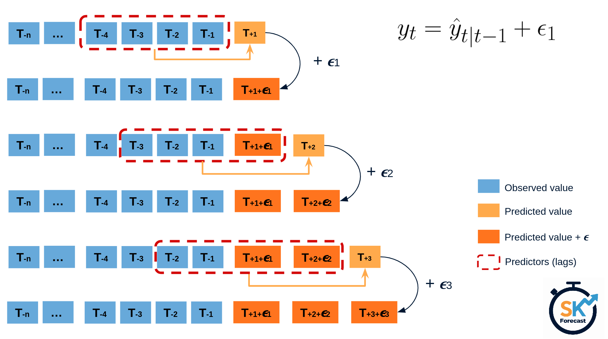
Doing this repeatedly, a collection of slightly different predictions is created (possible future paths), that represent the expected variance in the forecasting process.
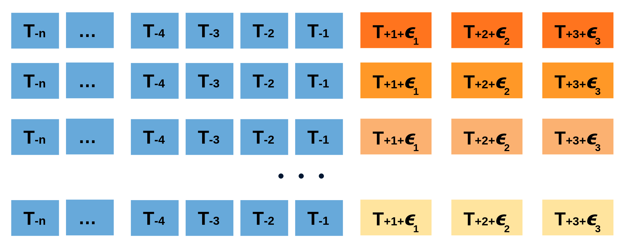
Finally, prediction intervals can be computed by calculating the $α/2$ and $1 − α/2$ percentiles of the simulated data at each forecasting horizon.
The main advantage of this strategy is that it only requires a single model to estimate any interval. The drawback is that, running hundreds or thousands of bootstrapping iterations, is computationally very expensive and not always workable.
This type of prediction intervals can be easily estimated using the method predict_interval of classes ForecasterAutoreg and ForecasterAutoregCustom models.
Prediction intervals using quantile regression models
As opposed to linear regression, which is intended to estimate the conditional mean of the response variable given certain values of the predictor variables, quantile regression aims at estimating the conditional quantiles of the response variable. For a continuous distribution function, the $\alpha$-quantile $Q_{\alpha}(x)$ is defined such that the probability of $Y$ being smaller than $Q_{\alpha}(x)$ is, for a given $X=x$, equal to $\alpha$. For example, 36% of the population values are lower than the quantile $Q=0.36$. The most known quantile is the 50%-quantile, more commonly called the median.
By combining the predictions of two quantile regressors, it is possible to build an interval. Each model estimates one of the limits of the interval. For example, the models obtained for $Q = 0.1$ and $Q = 0.9$ produce an 80% prediction interval (90% - 10% = 80%).
Several machine learning algorithms are capable of modeling quantiles. Some of them are:
Just as the squared-error loss function is used to train models that predict the mean value, a specific loss function is needed in order to train models that predict quantiles. The most common metric used for quantile regression is calles quantile loss or pinball loss:
$$\text{pinball}(y, \hat{y}) = \frac{1}{n_{\text{samples}}} \sum_{i=0}^{n_{\text{samples}}-1} \alpha \max(y_i - \hat{y}_i, 0) + (1 - \alpha) \max(\hat{y}_i - y_i, 0)$$where $\alpha$ is the target quantile, $y$ the real value and $\hat{y}$ the quantile prediction.
It can be seen that loss differs depending on the evaluated quantile. The higher the quantile, the more the loss function penalizes underestimates, and the less it penalizes overestimates. As with MSE and MAE, the goal is to minimize its values (the lower loss, the better).
Two disadvantages of quantile regression, compared to the bootstrap approach to prediction intervals, are that each quantile needs its regressor and quantile regression is not available for all types of regression models. However, once the models are trained, the inference is much faster since no iterative process is needed.
This type of prediction intervals can be easily estimated using quantile regressor inside a Forecaster object.
Libraries
Libraries used in this document.
# Data processing
# ==============================================================================
import numpy as np
import pandas as pd

# Plots
# ==============================================================================
import matplotlib.pyplot as plt
import matplotlib.ticker as ticker
from statsmodels.graphics.tsaplots import plot_acf
import plotly.express as px
import plotly.graph_objects as go
plt.style.use('fivethirtyeight')
plt.rcParams['lines.linewidth'] = 1.5
dark_style = {
    'figure.facecolor': '#212946',
    'axes.facecolor': '#212946',
    'savefig.facecolor':'#212946',
    'axes.grid': True,
    'axes.grid.which': 'both',
    'axes.spines.left': False,
    'axes.spines.right': False,
    'axes.spines.top': False,
    'axes.spines.bottom': False,
    'grid.color': '#2A3459',
    'grid.linewidth': '1',
    'text.color': '0.9',
    'axes.labelcolor': '0.9',
    'xtick.color': '0.9',
    'ytick.color': '0.9',
    'font.size': 12
}
plt.rcParams.update(dark_style)

# Modelling and Forecasting
# ==============================================================================
from lightgbm import LGBMRegressor
import sklearn.linear_model
from skforecast.ForecasterAutoreg import ForecasterAutoreg
from skforecast.ForecasterAutoregDirect import ForecasterAutoregDirect
from skforecast.model_selection import grid_search_forecaster
from skforecast.model_selection import backtesting_forecaster
from sklearn.metrics import mean_pinball_loss

# Configuration
# ==============================================================================
import warnings
warnings.filterwarnings('once')
Data
Data used in this document were obtained from the R tsibbledata package. The dataset contains half-hourly electricity demand for Victoria (Australia) and additional information about the temperature and an indicator for if that day is a public holiday. In the following examples, data are aggregated at the daily level.
# Data download
# ==============================================================================
url = ('https://raw.githubusercontent.com/JoaquinAmatRodrigo/skforecast/master/' +
       'data/vic_elec.csv')
data = pd.read_csv(url, sep=',')

# Data preparation (aggregation at daily level)
# ==============================================================================
data['Time'] = pd.to_datetime(data['Time'], format='%Y-%m-%dT%H:%M:%SZ')
data = data.set_index('Time')
data = data.asfreq('30min')
data = data.sort_index()
data = data.drop(columns='Date')
data = data.resample(rule='D', closed='left', label ='right')\
       .agg({'Demand': 'sum', 'Temperature': 'mean', 'Holiday': 'max'})
data.head()
# Split data into train-val-test
# ==============================================================================
data = data.loc['2012-01-01 00:00:00': '2014-12-30 23:00:00']
end_train = '2013-12-31 23:59:00'
end_validation = '2014-9-30 23:59:00'
data_train = data.loc[: end_train, :].copy()
data_val   = data.loc[end_train:end_validation, :].copy()
data_test  = data.loc[end_validation:, :].copy()

print(f"Train dates      : {data_train.index.min()} --- {data_train.index.max()}  (n={len(data_train)})")
print(f"Validation dates : {data_val.index.min()} --- {data_val.index.max()}  (n={len(data_val)})")
print(f"Test dates       : {data_test.index.min()} --- {data_test.index.max()}  (n={len(data_test)})")
# Plot time serie partition
# ==============================================================================
fig, ax=plt.subplots(figsize=(8, 4))
data_train['Demand'].plot(label='train', ax=ax)
data_val['Demand'].plot(label='validation', ax=ax)
data_test['Demand'].plot(label='test', ax=ax)
ax.yaxis.set_major_formatter(ticker.EngFormatter())
ax.set_ylim(bottom=160_000)
ax.set_ylabel('MW')
ax.set_title('Energy demand')
ax.legend();

# Interactive plot of time series
# ==============================================================================
# data.loc[:end_train, 'partition'] = 'train'
# data.loc[end_train:end_validation, 'partition'] = 'validation'
# data.loc[end_validation:, 'partition'] = 'test'

# fig = px.line(
#     data_frame = data.iloc[1:, :].reset_index(),
#     x      = 'Time',
#     y      = 'Demand',
#     color  = 'partition',
#     title  = 'Total demand per day',
#     width  = 900,
#     height = 500
# )

# fig.update_xaxes(
#     rangeslider_visible=True,
#     rangeselector=dict(
#         buttons=list([
#             dict(count=1, label="1m", step="month", stepmode="backward"),
#             dict(count=6, label="6m", step="month", stepmode="backward"),
#             dict(count=1, label="YTD", step="year", stepmode="todate"),
#             dict(count=1, label="1y", step="year", stepmode="backward"),
#             dict(step="all")
#         ])
#     )
# )

# fig.show()

# data=data.drop(columns='partition')
# Autocorrelation plot
# ==============================================================================
fig, ax = plt.subplots(figsize=(5, 2))
plot_acf(data.Demand, ax=ax, lags=30)
plt.show()

Base on the autocorrelation plot, the last 7 days may be used as predictors.
Bootstrapping prediction intervals
A recursive-multi-step forecaster is trained and its hyper-parameters optimized. Then, prediction intervals based on bootstrapped residuals are estimated.
# Create forecaster
# ==============================================================================
forecaster = ForecasterAutoreg(
                regressor = LGBMRegressor(),
                lags = 7
            )
forecaster
In order to find the best value for the hyper-parameters, a grid search is carried out. It is important not to include test data in the search, otherwise model overfitting could happen.
# Grid search of hyper-parameters and lags
# ==============================================================================
# Regressor hyper-parameters
param_grid = {
    'n_estimators': [100, 500],
    'max_depth': [3, 5, 10],
    'learning_rate': [0.01, 0.1]
}

# Lags used as predictors
lags_grid = [7]

results_grid_q10 = grid_search_forecaster(
                            forecaster         = forecaster,
                            y                  = data.loc[:end_validation, 'Demand'],
                            param_grid         = param_grid,
                            lags_grid          = lags_grid,
                            steps              = 7,
                            refit              = False,
                            metric             = 'mean_squared_error',
                            initial_train_size = int(len(data_train)),
                            fixed_train_size   = False,
                            return_best        = True,
                            n_jobs             = 'auto',
                            verbose            = False,
                            show_progress      = True
                    )
Once the best hyper-parameters have been found, a backtesting process is applied in order to evaluate the forecaster's performance on test data and calculate the real coverage of the estimated interval.
# Backtesting
# ==============================================================================
metric, predictions = backtesting_forecaster(
                            forecaster = forecaster,
                            y          = data['Demand'],
                            initial_train_size = len(data_train) + len(data_val),
                            fixed_train_size   = False,
                            steps              = 7,
                            refit              = False,
                            interval           = [10, 90],
                            n_boot             = 1000,
                            metric             = 'mean_squared_error',
                            verbose            = False,
                            show_progress      = True
                        )
predictions.head(4)
# Interval coverage on test data
# ==============================================================================
inside_interval = np.where(
                     (data.loc[predictions.index, 'Demand'] >= predictions['lower_bound']) & \
                     (data.loc[predictions.index, 'Demand'] <= predictions['upper_bound']),
                     True,
                     False
                  )

coverage = inside_interval.mean()
print(f"Coverage of the predicted interval on test data: {100 * coverage}")
The coverage of the predicted interval (71%) is lower than the expected (80%).
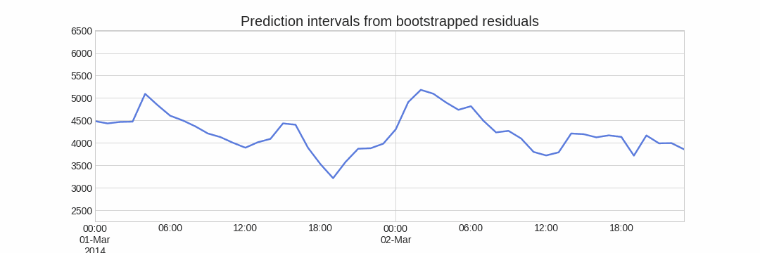
# Static plot
# ==============================================================================
fig, ax=plt.subplots(figsize=(8, 3))
data.loc[end_validation:, 'Demand'].plot(ax=ax, label='Demand', linewidth=3, color="#23b7ff")
ax.fill_between(
    predictions.index,
    predictions['lower_bound'],
    predictions['upper_bound'],
    color = 'deepskyblue',
    alpha = 0.3,
    label = '80% interval'
)
ax.yaxis.set_major_formatter(ticker.EngFormatter())
ax.set_ylabel('MW')
ax.set_title('Energy demand forecast')
ax.legend();

# Interactive plot
# ==============================================================================
# fig = px.line(
#     data_frame = data.loc[end_validation:, 'Demand'].reset_index(),
#     x      = 'Time',
#     y      = 'Demand',
#     title  = 'Total demand per day',
#     width  = 900,
#     height = 500
# )

# fig.add_traces([
#     go.Scatter(
#         x = predictions.index,
#         y = predictions['lower_bound'],
#         mode = 'lines',
#         line_color = 'rgba(0,0,0,0)',
#         showlegend = False
#     ),
#     go.Scatter(
#         x = predictions.index,
#         y = predictions['upper_bound'],
#         mode = 'lines',
#         line_color = 'rgba(0,0,0,0)',
#         fill='tonexty',
#         fillcolor = 'rgba(255, 0, 0, 0.2)',
#         showlegend = False
#     )]
# )

# fig.show()
By default, training residuals are used to create the prediction intervals. However, other residuals can be used, for example, residuals obtained from a validation set.
To do this, the new residuals must be stored inside the forecaster using the set_out_sample_residuals method. Once the new residuals have been added to the forecaster, set in_sample_residuals = False when using the predict_interval method.
Quantile regresion models
As in the previous example, an 80% prediction interval is estimated for 7 steps-ahead predictions but, this time, using quantile regression. A LightGBM gradient boosting model is trained in this example, however, the reader may use any other model just replacing the definition of the regressor.
# Create forecasters: one for each limit of the interval
# ==============================================================================
# The forecasters obtained for alpha=0.1 and alpha=0.9 produce a 80% confidence
# interval (90% - 10% = 80%).

# Forecaster for quantile 10%
forecaster_q10 = ForecasterAutoregDirect(
                    regressor = LGBMRegressor(
                                    objective     = 'quantile',
                                    metric        = 'quantile',
                                    alpha         = 0.1,
                                    learning_rate = 0.1,
                                    max_depth     = 10,
                                    n_estimators  = 100
                                ),
                    lags = 7,
                    steps = 7
                  )
# Forecaster for quantile 90%
forecaster_q90 = ForecasterAutoregDirect(
                    regressor = LGBMRegressor(
                                    objective     = 'quantile',
                                    metric        = 'quantile',
                                    alpha         = 0.9,
                                    learning_rate = 0.1,
                                    max_depth     = 10,
                                    n_estimators  = 100
                                ),
                    lags = 7,
                    steps = 7
                  )
When validating a quantile regression model, a custom metric must be provided depending on the quantile being estimated. These metrics will be used again when tuning the hyper-parameters of each model.
# Loss function for each quantile (pinball_loss)
# ==============================================================================
def mean_pinball_loss_q10(y_true, y_pred):
    '''
    Pinball loss for quantile 10.
    '''
    return mean_pinball_loss(y_true, y_pred, alpha=0.1)


def mean_pinball_loss_q90(y_true, y_pred):
    '''
    Pinball loss for quantile 90.
    '''
    return mean_pinball_loss(y_true, y_pred, alpha=0.9)
# Backtesting on test data
# ==============================================================================
metric_q10, predictions_q10 = backtesting_forecaster(
                                    forecaster = forecaster_q10,
                                    y          = data['Demand'],
                                    initial_train_size = len(data_train) + len(data_val),
                                    fixed_train_size   = False,
                                    steps      = 7,
                                    refit      = False,
                                    metric     = mean_pinball_loss_q10,
                                    verbose    = False
                                )

metric_q90, predictions_q90 = backtesting_forecaster(
                                    forecaster = forecaster_q90,
                                    y          = data['Demand'],
                                    initial_train_size = len(data_train) + len(data_val),
                                    fixed_train_size   = False,
                                    steps      = 7,
                                    refit      = False,
                                    metric     = mean_pinball_loss_q90,
                                    verbose    = False
                                )
Predictions generated for each model are used to define the upper and lower limits of the interval.
# Interval coverage on test data
# ==============================================================================
inside_interval = np.where(
                     (data.loc[end_validation:, 'Demand'] >= predictions_q10['pred']) & \
                     (data.loc[end_validation:, 'Demand'] <= predictions_q90['pred']),
                     True,
                     False
                   )

coverage = inside_interval.mean()
print(f"Coverage of the predicted interval: {100 * coverage}")
The coverage of the predicted interval (56%) is much lower than the expected (80%).
The hyper-parameters of the model were hand-tuned and there is no reason that the same hyper-parameters are suitable for the 10th and 90th percentiles regressors. Therefore, a grid search is carried out for each forecaster.
# Grid search of hyper-parameters and lags for each quantile forecaster
# ==============================================================================
# Regressor hyper-parameters
param_grid = {
    'n_estimators': [100, 500],
    'max_depth': [3, 5, 10],
    'learning_rate': [0.01, 0.1]
}

# Lags used as predictors
lags_grid = [7]

results_grid_q10 = grid_search_forecaster(
                            forecaster         = forecaster_q10,
                            y                  = data.loc[:end_validation, 'Demand'],
                            param_grid         = param_grid,
                            lags_grid          = lags_grid,
                            steps              = 7,
                            refit              = False,
                            metric             = mean_pinball_loss_q10,
                            initial_train_size = int(len(data_train)),
                            fixed_train_size   = False,
                            return_best        = True,
                            verbose            = False,
                            show_progress      = False
                    )

results_grid_q90 = grid_search_forecaster(
                            forecaster         = forecaster_q90,
                            y                  = data.loc[:end_validation, 'Demand'],
                            param_grid         = param_grid,
                            lags_grid          = lags_grid,
                            steps              = 7,
                            refit              = False,
                            metric             = mean_pinball_loss_q90,
                            initial_train_size = int(len(data_train)),
                            fixed_train_size   = False,
                            return_best        = True,
                            verbose            = False,
                            show_progress      = False
                    )
Once the best hyper-parameters have been found for each forecaster, a backtesting process is applied again using the test data.
# Backtesting on test data
# ==============================================================================
metric_q10, predictions_q10 = backtesting_forecaster(
                                    forecaster = forecaster_q10,
                                    y          = data['Demand'],
                                    initial_train_size = len(data_train) + len(data_val),
                                    fixed_train_size   = False,
                                    steps      = 7,
                                    refit      = False,
                                    metric     = mean_pinball_loss_q10,
                                    verbose    = False
                                )

metric_q90, predictions_q90 = backtesting_forecaster(
                                    forecaster = forecaster_q90,
                                    y          = data['Demand'],
                                    initial_train_size = len(data_train) + len(data_val),
                                    fixed_train_size   = False,
                                    steps      = 7,
                                    refit      = False,
                                    metric     = mean_pinball_loss_q90,
                                    verbose    = False
                                )
# Plot
# ==============================================================================
fig, ax=plt.subplots(figsize=(8, 3))
data.loc[end_validation:, 'Demand'].plot(ax=ax, label='Demand', linewidth=3, color="#23b7ff")
ax.fill_between(
    data.loc[end_validation:].index,
    predictions_q10['pred'],
    predictions_q90['pred'],
    color = 'deepskyblue',
    alpha = 0.3,
    label = '80% interval'
)
ax.yaxis.set_major_formatter(ticker.EngFormatter())
ax.set_ylabel('MW')
ax.set_title('Energy demand forecast')
ax.legend();

# Interval coverage
# ==============================================================================
inside_interval = np.where(
                     (data.loc[end_validation:, 'Demand'] >= predictions_q10['pred']) & \
                     (data.loc[end_validation:, 'Demand'] <= predictions_q90['pred']),
                     True,
                     False
                   )

coverage = inside_interval.mean()
print(f"Coverage of the predicted interval: {100 * coverage}")
After optimizing the hyper-parameters of each quantile forecaster, the coverage is closer to the expected one (80%).
Session information
import session_info
session_info.show(html=False)
How to cite this document?
Prediction intervals when forecasting with machine learning models by Joaquín Amat Rodrigo and Javier Escobar Ortiz, available under a CC BY-NC-SA 4.0 at https://www.cienciadedatos.net/py42-forecasting-prediction-intervals-machine-learning.html ![]()
Did you like the article? Your support is important
Website maintenance has high cost, your contribution will help me to continue generating free educational content. Many thanks! 😊

This work by Joaquín Amat Rodrigo and Javier Escobar Ortiz is licensed under a Attribution-NonCommercial-ShareAlike 4.0 International.