More about forecasting in cienciadedatos.net
- ARIMA and SARIMAX models with python
- Time series forecasting with machine learning
- Forecasting time series with gradient boosting: XGBoost, LightGBM and CatBoost
- Forecasting time series with XGBoost
- Global Forecasting Models: Multi-series forecasting
- Global Forecasting Models: Comparative Analysis of Single and Multi-Series Forecasting Modeling
- Probabilistic forecasting
- Forecasting with deep learning
- Forecasting energy demand with machine learning
- Forecasting web traffic with machine learning
- Intermittent demand forecasting
- Modelling time series trend with tree-based models
- Bitcoin price prediction with Python
- Stacking ensemble of machine learning models to improve forecasting
- Interpretable forecasting models
- Mitigating the Impact of Covid on forecasting Models
- Forecasting time series with missing values

Introduction
In Single-Series Modeling (Local Forecasting Model), each time series is analyzed individually, modeled as a combination of its own lags and, optionally, exogenous variables. This approach provides detailed insights specific to each series but can become impractical for scaling when dealing with a large number of time series. In contrast, Multi-Series Modeling (Global Forecasting Model) involves building a unified predictive model that learns multiple time series simultaneously. It attempts to capture common dynamics that influence the series as a whole, thereby reducing noise from individual series. This approach is computationally efficient, easy to maintain, and can yield more robust generalizations across time series, albeit potentially at the cost of sacrificing some individual insights. Two strategies of global forecasting models can be distinguished: Independent multi-series and dependent multi-series.
Advantages of multi-series:
It is easier to maintain and monitor a single model than several.
Since all time series are combined during training, the model has a higher learning capacity even if the series are short.
By combining multiple time series, the model can learn more generalizable patterns.
Limitations of multi-series:
If the series do not follow the same internal dynamics, the model may learn a pattern that does not represent any of them.
The series may mask each other, so the model may not predict all of them with the same performance.
It is more computationally demanding (time and resources) to train and backtest a big model than several small ones.
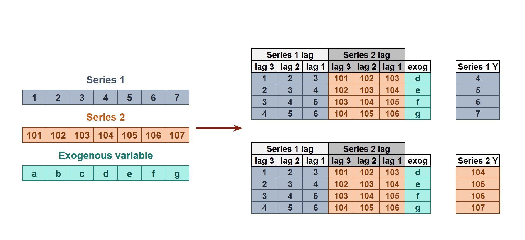
Dependent multi-series forecasting (Multivariate forecasting)
In dependent multi-series forecasting (multivariate time series), all series are modeled together in a single model, considering that each time series depends not only on its past values but also on the past values of the other series. The forecaster is expected not only to learn the information of each series separately but also to relate them. An example is the measurements made by all the sensors (flow, temperature, pressure...) installed on an industrial machine such as a compressor.
💡 Tip
This is part of a series of documents on global forecasting models:- Global Forecasting Models: Modeling multiple time series with machine learning
- Scalable Forecasting: modeling thousand time series with a single global model
- Global Forecasting Models: Comparative Analysis of Single and Multi-Series Forecasting Modeling
- A Step-by-Step Guide to Global Time Series Forecasting Using Kaggle Sticker Sales Data
- The M5 Accuracy competition: the success of global forecasting models
- Clustering Time Series to Improve Forecasting Models
- Forecasting at scale with deep learning models
Multiple time series with equal length
In this first example, multiple time series with the same length are used. The goal is to compare the forecasting results of a global model with those of an individual model for each series when forecasting the next 7 days of sales for 50 different items in a store using the 5 years of available history. The data has been obtained from the Store Item Demand Forecasting Challenge. This dataset contains 913,000 sales transactions from 01/01/2013 to 31/12/2017 for 50 products (SKU) in 10 stores.
Libraries
# Data manipulation
# ==============================================================================
import numpy as np
import pandas as pd
# Plots
# ==============================================================================
import matplotlib.pyplot as plt
from skforecast.plot import set_dark_theme
from tqdm.notebook import tqdm
# Modelling and Forecasting
# ==============================================================================
import sklearn
import skforecast
from sklearn.ensemble import HistGradientBoostingRegressor
from sklearn.preprocessing import StandardScaler
from skforecast.recursive import ForecasterRecursive, ForecasterRecursiveMultiSeries
from skforecast.model_selection import (
TimeSeriesFold,
OneStepAheadFold,
backtesting_forecaster,
bayesian_search_forecaster,
backtesting_forecaster_multiseries,
bayesian_search_forecaster_multiseries
)
from skforecast.preprocessing import (
RollingFeatures,
reshape_series_long_to_dict,
reshape_exog_long_to_dict
)
from skforecast.exceptions import OneStepAheadValidationWarning
# Warnings configuration
# ==============================================================================
import warnings
color = "\033[1m\033[38;5;208m"
print(f"{color}Version skforecast: {skforecast.__version__}")
print(f"{color}Version scikit-learn: {sklearn.__version__}")
print(f"{color}Version pandas: {pd.__version__}")
print(f"{color}Version numpy: {np.__version__}")
Version skforecast: 0.22.0 Version scikit-learn: 1.7.2 Version pandas: 2.3.3 Version numpy: 2.1.3
Data
# Data loading
# ======================================================================================
data = pd.read_csv('./train_stores_kaggle.csv')
display(data)
print(f"Shape: {data.shape}")
| date | store | item | sales | |
|---|---|---|---|---|
| 0 | 2013-01-01 | 1 | 1 | 13 |
| 1 | 2013-01-02 | 1 | 1 | 11 |
| 2 | 2013-01-03 | 1 | 1 | 14 |
| 3 | 2013-01-04 | 1 | 1 | 13 |
| 4 | 2013-01-05 | 1 | 1 | 10 |
| ... | ... | ... | ... | ... |
| 912995 | 2017-12-27 | 10 | 50 | 63 |
| 912996 | 2017-12-28 | 10 | 50 | 59 |
| 912997 | 2017-12-29 | 10 | 50 | 74 |
| 912998 | 2017-12-30 | 10 | 50 | 62 |
| 912999 | 2017-12-31 | 10 | 50 | 82 |
913000 rows × 4 columns
Shape: (913000, 4)
# Data preprocessing
# ======================================================================================
selected_store = 2
selected_items = data.item.unique()
data = data[(data['store'] == selected_store) & (data['item'].isin(selected_items))].copy()
data['date'] = pd.to_datetime(data['date'], format='%Y-%m-%d')
data = pd.pivot_table(
data = data,
values = 'sales',
index = 'date',
columns = 'item'
)
data.columns.name = None
data.columns = [f"item_{col}" for col in data.columns]
data = data.asfreq('1D')
data = data.sort_index()
data.head(4)
| item_1 | item_2 | item_3 | item_4 | item_5 | item_6 | item_7 | item_8 | item_9 | item_10 | ... | item_41 | item_42 | item_43 | item_44 | item_45 | item_46 | item_47 | item_48 | item_49 | item_50 | |
|---|---|---|---|---|---|---|---|---|---|---|---|---|---|---|---|---|---|---|---|---|---|
| date | |||||||||||||||||||||
| 2013-01-01 | 12.0 | 41.0 | 19.0 | 21.0 | 4.0 | 34.0 | 39.0 | 49.0 | 28.0 | 51.0 | ... | 11.0 | 25.0 | 36.0 | 12.0 | 45.0 | 43.0 | 12.0 | 45.0 | 29.0 | 43.0 |
| 2013-01-02 | 16.0 | 33.0 | 32.0 | 14.0 | 6.0 | 40.0 | 47.0 | 42.0 | 21.0 | 56.0 | ... | 19.0 | 21.0 | 35.0 | 25.0 | 50.0 | 52.0 | 13.0 | 37.0 | 25.0 | 57.0 |
| 2013-01-03 | 16.0 | 46.0 | 26.0 | 12.0 | 12.0 | 41.0 | 43.0 | 46.0 | 29.0 | 46.0 | ... | 23.0 | 20.0 | 52.0 | 18.0 | 56.0 | 30.0 | 5.0 | 45.0 | 30.0 | 45.0 |
| 2013-01-04 | 20.0 | 50.0 | 34.0 | 17.0 | 16.0 | 41.0 | 44.0 | 55.0 | 32.0 | 56.0 | ... | 15.0 | 28.0 | 50.0 | 24.0 | 57.0 | 46.0 | 19.0 | 32.0 | 20.0 | 45.0 |
4 rows × 50 columns
The dataset is divided into 3 partitions: one for training, one for validation, and one for testing.
# Split data into train-validation-test
# ======================================================================================
end_train = '2016-05-31 23:59:00'
end_val = '2017-05-31 23:59:00'
data_train = data.loc[:end_train, :].copy()
data_val = data.loc[end_train:end_val, :].copy()
data_test = data.loc[end_val:, :].copy()
print(f"Train dates : {data_train.index.min()} --- {data_train.index.max()} (n={len(data_train)})")
print(f"Validation dates : {data_val.index.min()} --- {data_val.index.max()} (n={len(data_val)})")
print(f"Test dates : {data_test.index.min()} --- {data_test.index.max()} (n={len(data_test)})")
Train dates : 2013-01-01 00:00:00 --- 2016-05-31 00:00:00 (n=1247) Validation dates : 2016-06-01 00:00:00 --- 2017-05-31 00:00:00 (n=365) Test dates : 2017-06-01 00:00:00 --- 2017-12-31 00:00:00 (n=214)
Four of the series are plotted to understand their trends and patterns. The reader is strongly encouraged to plot several more to gain an in-depth understanding of the series.
# Plot time series
# ======================================================================================
set_dark_theme()
fig, axs = plt.subplots(4, 1, figsize=(7, 5), sharex=True)
data.iloc[:, :4].plot(
legend = True,
subplots = True,
title = 'Sales of store 2',
ax = axs,
linewidth = 1
)
for ax in axs:
ax.axvline(pd.to_datetime(end_train) , color='white', linestyle='--', linewidth=1.5)
ax.axvline(pd.to_datetime(end_val) , color='white', linestyle='--', linewidth=1.5)
fig.tight_layout()
plt.show()

Individual Forecaster for each product
A separate Gradient Boosting Machine (GBM) model is trained for each item, using sales over the last 14 days, as well as the average, maximum and minimum sales over the last 7 days as predictive features. The performance of the model over the next 7 days is evaluated using backtesting with the Mean Absolute Error (MAE) as the evaluation metric. Finally, the performance of these individual models is compared with that of a global model trained on all series.
# Train and backtest a model for each item: ForecasterRecursive
# ======================================================================================
items = []
mae_values = []
predictions = {}
for i, item in enumerate(tqdm(data.columns)):
# Define forecaster
window_features = RollingFeatures(stats=['mean', 'min', 'max'], window_sizes=7)
forecaster = ForecasterRecursive(
estimator = HistGradientBoostingRegressor(random_state=8523),
lags = 14,
window_features = window_features
)
# Backtesting forecaster
cv = TimeSeriesFold(
steps = 7,
initial_train_size = len(data_train) + len(data_val),
refit = False,
)
metric, preds = backtesting_forecaster(
forecaster = forecaster,
y = data[item],
cv = cv,
metric = 'mean_absolute_error',
show_progress = False
)
items.append(item)
mae_values.append(metric.at[0, 'mean_absolute_error'])
predictions[item] = preds
# Results
uni_series_mae = pd.Series(
data = mae_values,
index = items,
name = 'uni_series_mae'
)
uni_series_mae.head()
item_1 6.004406 item_2 9.994352 item_3 8.652751 item_4 5.528955 item_5 5.096925 Name: uni_series_mae, dtype: float64
Global model
A global model is trained on all series simultaneously and evaluated using the same backtesting process as the individual models.
# Train and backtest a model for all items: ForecasterRecursiveMultiSeries
# ======================================================================================
items = list(data.columns)
# Define forecaster
window_features = RollingFeatures(stats=['mean', 'min', 'max'], window_sizes=7)
forecaster_ms = ForecasterRecursiveMultiSeries(
estimator = HistGradientBoostingRegressor(random_state=8523),
lags = 14,
encoding = 'ordinal',
transformer_series = StandardScaler(),
window_features = window_features,
)
# Backtesting forecaster for all items
cv = TimeSeriesFold(
steps = 7,
initial_train_size = len(data_train) + len(data_val),
refit = False,
)
multi_series_mae, predictions_ms = backtesting_forecaster_multiseries(
forecaster = forecaster_ms,
series = data,
levels = items,
cv = cv,
metric = 'mean_absolute_error',
)
# Results
display(multi_series_mae.head(3))
print('')
display(predictions_ms.head(3))
╭────────────────────────────────── InputTypeWarning ──────────────────────────────────╮ │ Passing a DataFrame (either wide or long format) as `series` requires additional │ │ internal transformations, which can increase computational time. It is recommended │ │ to use a dictionary of pandas Series instead. For more details, see: │ │ https://skforecast.org/latest/user_guides/independent-multi-time-series-forecasting. │ │ html#input-data │ │ │ │ Category : skforecast.exceptions.InputTypeWarning │ │ Location : │ │ /home/ubuntu/anaconda3/envs/skforecast_22_py13/lib/python3.13/site-packages/skforeca │ │ st/utils/utils.py:2802 │ │ Suppress : warnings.simplefilter('ignore', category=InputTypeWarning) │ ╰──────────────────────────────────────────────────────────────────────────────────────╯
| levels | mean_absolute_error | |
|---|---|---|
| 0 | item_1 | 5.521236 |
| 1 | item_2 | 9.245126 |
| 2 | item_3 | 7.301948 |
| level | fold | pred | |
|---|---|---|---|
| 2017-06-01 | item_1 | 0 | 35.106861 |
| 2017-06-01 | item_2 | 0 | 90.367217 |
| 2017-06-01 | item_3 | 0 | 60.613740 |
Comparison
The mean absolute error (MAE) for each item is calculated using the individual and global models. The results are compared to determine which model performs better.
# Difference of backtesting metric for each item
# ======================================================================================
multi_series_mae = multi_series_mae.set_index('levels')
multi_series_mae.columns = ['multi_series_mae']
results = pd.concat((uni_series_mae, multi_series_mae), axis = 1)
results['improvement'] = results.eval('uni_series_mae - multi_series_mae')
results['improvement_(%)'] = 100 * results.eval('(uni_series_mae - multi_series_mae) / uni_series_mae')
results = results.round(2)
results.style.bar(subset=['improvement_(%)'], align='mid', color=['#d65f5f', '#5fba7d'])
| uni_series_mae | multi_series_mae | improvement | improvement_(%) | |
|---|---|---|---|---|
| item_1 | 6.000000 | 5.520000 | 0.480000 | 8.050000 |
| item_2 | 9.990000 | 9.250000 | 0.750000 | 7.500000 |
| item_3 | 8.650000 | 7.300000 | 1.350000 | 15.610000 |
| item_4 | 5.530000 | 5.030000 | 0.500000 | 8.960000 |
| item_5 | 5.100000 | 4.660000 | 0.440000 | 8.630000 |
| item_6 | 10.830000 | 9.750000 | 1.080000 | 9.960000 |
| item_7 | 10.580000 | 9.830000 | 0.750000 | 7.120000 |
| item_8 | 11.810000 | 10.420000 | 1.400000 | 11.830000 |
| item_9 | 9.420000 | 8.690000 | 0.730000 | 7.760000 |
| item_10 | 11.640000 | 10.330000 | 1.300000 | 11.210000 |
| item_11 | 11.520000 | 10.430000 | 1.090000 | 9.450000 |
| item_12 | 11.960000 | 10.890000 | 1.080000 | 8.990000 |
| item_13 | 12.130000 | 11.360000 | 0.760000 | 6.300000 |
| item_14 | 10.350000 | 9.560000 | 0.790000 | 7.610000 |
| item_15 | 12.460000 | 11.640000 | 0.820000 | 6.620000 |
| item_16 | 6.000000 | 5.920000 | 0.090000 | 1.480000 |
| item_17 | 7.460000 | 7.190000 | 0.270000 | 3.560000 |
| item_18 | 12.690000 | 12.120000 | 0.570000 | 4.490000 |
| item_19 | 7.720000 | 7.370000 | 0.360000 | 4.600000 |
| item_20 | 8.250000 | 7.830000 | 0.420000 | 5.080000 |
| item_21 | 8.580000 | 8.060000 | 0.520000 | 6.080000 |
| item_22 | 11.790000 | 10.710000 | 1.080000 | 9.150000 |
| item_23 | 7.490000 | 6.770000 | 0.720000 | 9.600000 |
| item_24 | 10.470000 | 9.860000 | 0.610000 | 5.850000 |
| item_25 | 12.950000 | 11.650000 | 1.310000 | 10.100000 |
| item_26 | 9.230000 | 8.590000 | 0.640000 | 6.930000 |
| item_27 | 5.480000 | 5.170000 | 0.310000 | 5.680000 |
| item_28 | 12.590000 | 12.080000 | 0.510000 | 4.020000 |
| item_29 | 10.980000 | 10.180000 | 0.810000 | 7.330000 |
| item_30 | 8.430000 | 7.890000 | 0.530000 | 6.290000 |
| item_31 | 10.530000 | 10.070000 | 0.460000 | 4.420000 |
| item_32 | 9.710000 | 9.160000 | 0.540000 | 5.580000 |
| item_33 | 9.740000 | 9.320000 | 0.420000 | 4.270000 |
| item_34 | 6.340000 | 5.930000 | 0.410000 | 6.450000 |
| item_35 | 11.200000 | 10.180000 | 1.020000 | 9.120000 |
| item_36 | 12.000000 | 10.620000 | 1.380000 | 11.520000 |
| item_37 | 6.510000 | 6.110000 | 0.400000 | 6.150000 |
| item_38 | 11.620000 | 11.130000 | 0.500000 | 4.270000 |
| item_39 | 8.340000 | 7.370000 | 0.970000 | 11.680000 |
| item_40 | 7.100000 | 6.630000 | 0.470000 | 6.650000 |
| item_41 | 5.670000 | 5.220000 | 0.450000 | 7.950000 |
| item_42 | 7.440000 | 6.940000 | 0.500000 | 6.680000 |
| item_43 | 8.620000 | 8.570000 | 0.050000 | 0.540000 |
| item_44 | 6.980000 | 6.410000 | 0.570000 | 8.190000 |
| item_45 | 12.720000 | 11.790000 | 0.930000 | 7.310000 |
| item_46 | 10.350000 | 9.890000 | 0.460000 | 4.450000 |
| item_47 | 5.500000 | 4.980000 | 0.520000 | 9.500000 |
| item_48 | 9.270000 | 8.190000 | 1.090000 | 11.740000 |
| item_49 | 6.300000 | 5.960000 | 0.340000 | 5.350000 |
| item_50 | 11.860000 | 10.610000 | 1.250000 | 10.510000 |
| average | nan | 8.620000 | nan | nan |
| weighted_average | nan | 8.620000 | nan | nan |
| pooling | nan | 8.620000 | nan | nan |
# Average improvement for all items
# ======================================================================================
results[['improvement', 'improvement_(%)']].agg(['mean', 'min', 'max'])
| improvement | improvement_(%) | |
|---|---|---|
| mean | 0.696 | 7.3634 |
| min | 0.050 | 0.5400 |
| max | 1.400 | 15.6100 |
# Number of series with positive and negative improvement
# ======================================================================================
pd.Series(np.where(results['improvement_(%)'] < 0, 'negative', 'positive')).value_counts()
positive 53 Name: count, dtype: int64
The global model achieves an average improvement of 7.4% compared to using an individual model for each series. For all series, the prediction error evaluated by backtesting is lower when the global model is used. This use case demonstrates that a multi-series model can have advantages over multiple individual models when forecasting time series that follow similar dynamics. In addition to the potential improvements in forecasting, it is also important to consider the benefit of having only one model to maintain and the speed of training and prediction.
⚠️ Warning
This comparison was made without optimizing the model hyperparameters. See the Hyperparameter tuning and lags selection section to verify that the conclusions hold when the models are tuned with the best combination of hyperparameters and lags.
Series with different lengths and different exogenous variables
When faced with a multi-series forecasting problem, it is common for the series to have varying lengths due to differences in the starting times of data recording. To address this scenario, the ForecasterRecursiveMultiSeries allow the simultaneous modeling of time series of different lengths and using different exogenous variables. In these cases, the data must be structured in one of the following ways:
In a python
dictionaryofpandas.Series: the keys of the dictionary are the names of the series and the values are the series themselves. All series must be of typepandas.Series, have aDatetimeIndexindex, and have the same frequency.In a
pandas.DataFramewithMultiIndex: where the first level of the index contains the series name and the second level is the time index. All series must be of typepandas.Series, have aDatetimeIndexindex, and have the same frequency. This option is available starting from version0.17.0of skforecast.
| Series values | Allowed |
|---|---|
[NaN, NaN, NaN, NaN, 4, 5, 6, 7, 8, 9] |
✔️ |
[0, 1, 2, 3, 4, 5, 6, 7, 8, NaN] |
✔️ |
[0, 1, 2, 3, 4, NaN, 6, 7, 8, 9] |
✔️ |
[NaN, NaN, 2, 3, 4, NaN, 6, 7, 8, 9] |
✔️ |
When different exogenous variables are used for each series, or if the exogenous variables are the same but have different values for each series, they must be stored in one of the following ways:
In a dictionary: The keys of the dictionary are the names of the series and the values are the exogenous variables themselves. All exogenous variables must be of type
pandas.DataFrameorpandas.Series.In a
pandas.DataFramewithMultiIndex: where the first level of the index contains the series name and the second level is the time index. All exogenous variables must be of typepandas.DataFrameorpandas.Series.
If the data does not follow these structures, skforecast provides two functions to transform the data: reshape_series_long_to_dict and reshape_exog_long_to_dict.
💡 Tip
In terms of performance, using a dictionary is more efficient than a pandas DataFrame, either wide or long format, especially for larger datasets. This is because dictionaries enable faster access and manipulation of individual time series, without the structural overhead associated with DataFrames.
Data
The data for this example is stored in "long format" in a single DataFrame. The series_id column identifies the series to which each observation belongs. The timestamp column contains the date of the observation, and the value column contains the value of the series at that date. Each time series is of a different length. The exogenous variables are stored in a separate DataFrame, also in "long format". The column series_id identifies the series to which each observation belongs. The column timestamp contains the date of the observation, and the remaining columns contain the values of the exogenous variables at that date.
# Load time series of multiple lengths and exogenous variables
# ==============================================================================
series = pd.read_csv(
'https://raw.githubusercontent.com/skforecast/skforecast-datasets/main/data/demo_multi_series.csv'
)
exog = pd.read_csv(
'https://raw.githubusercontent.com/skforecast/skforecast-datasets/main/data/demo_multi_series_exog.csv'
)
series['timestamp'] = pd.to_datetime(series['timestamp'])
exog['timestamp'] = pd.to_datetime(exog['timestamp'])
display(series.head())
print("")
display(exog.head())
| series_id | timestamp | value | |
|---|---|---|---|
| 0 | id_1000 | 2016-01-01 | 1012.500694 |
| 1 | id_1000 | 2016-01-02 | 1158.500099 |
| 2 | id_1000 | 2016-01-03 | 983.000099 |
| 3 | id_1000 | 2016-01-04 | 1675.750496 |
| 4 | id_1000 | 2016-01-05 | 1586.250694 |
| series_id | timestamp | sin_day_of_week | cos_day_of_week | air_temperature | wind_speed | |
|---|---|---|---|---|---|---|
| 0 | id_1000 | 2016-01-01 | -0.433884 | -0.900969 | 6.416639 | 4.040115 |
| 1 | id_1000 | 2016-01-02 | -0.974928 | -0.222521 | 6.366474 | 4.530395 |
| 2 | id_1000 | 2016-01-03 | -0.781831 | 0.623490 | 6.555272 | 3.273064 |
| 3 | id_1000 | 2016-01-04 | 0.000000 | 1.000000 | 6.704778 | 4.865404 |
| 4 | id_1000 | 2016-01-05 | 0.781831 | 0.623490 | 2.392998 | 5.228913 |
When series have different lengths, the data must be transformed into a dictionary. The keys of the dictionary are the names of the series and the values are the series themselves. To do this, the reshape_series_long_to_dict function is used, which takes the DataFrame in "long format" and returns a dict of series.
Similarly, when the exogenous variables are different (values or variables) for each series, the data must be transformed into a dictionary. The keys of the dictionary are the names of the series and the values are the exogenous variables themselves. The reshape_exog_long_to_dict function is used, which takes the DataFrame in "long format" and returns a dict of exogenous variables.
# Transform series and exog to dictionaries
# ==============================================================================
series_dict = reshape_series_long_to_dict(
data = series,
series_id = 'series_id',
index = 'timestamp',
values = 'value',
freq = 'D'
)
exog_dict = reshape_exog_long_to_dict(
data = exog,
series_id = 'series_id',
index = 'timestamp',
freq = 'D'
)
╭──────────────────────────────── MissingValuesWarning ────────────────────────────────╮ │ Series 'id_1003' is incomplete. NaNs have been introduced after setting the │ │ frequency. │ │ │ │ Category : skforecast.exceptions.MissingValuesWarning │ │ Location : │ │ /home/ubuntu/anaconda3/envs/skforecast_22_py13/lib/python3.13/site-packages/skforeca │ │ st/preprocessing/preprocessing.py:534 │ │ Suppress : warnings.simplefilter('ignore', category=MissingValuesWarning) │ ╰──────────────────────────────────────────────────────────────────────────────────────╯
Some exogenous variables are omitted for series 1 and 3 to illustrate that different exogenous variables can be used for each series.
# Drop some exogenous variables for series 'id_1000' and 'id_1003'
# ==============================================================================
exog_dict['id_1000'] = exog_dict['id_1000'].drop(columns=['air_temperature', 'wind_speed'])
exog_dict['id_1003'] = exog_dict['id_1003'].drop(columns=['cos_day_of_week'])
# Partition data in train and test
# ==============================================================================
end_train = '2016-07-31 23:59:00'
series_dict_train = {k: v.loc[: end_train,] for k, v in series_dict.items()}
exog_dict_train = {k: v.loc[: end_train,] for k, v in exog_dict.items()}
series_dict_test = {k: v.loc[end_train:,] for k, v in series_dict.items()}
exog_dict_test = {k: v.loc[end_train:,] for k, v in exog_dict.items()}
# Plot series
# ==============================================================================
set_dark_theme()
colors = plt.rcParams['axes.prop_cycle'].by_key()['color']
fig, axs = plt.subplots(5, 1, figsize=(8, 4), sharex=True)
for i, s in enumerate(series_dict.values()):
axs[i].plot(s, label=s.name, color=colors[i])
axs[i].legend(loc='upper right', fontsize=8)
axs[i].tick_params(axis='both', labelsize=8)
axs[i].axvline(pd.to_datetime(end_train), color='white', linestyle='--', linewidth=1) # End train

# Description of each series
# ==============================================================================
for k in series_dict.keys():
print(f"{k}:")
try:
print(
f"\tTrain: len={len(series_dict_train[k])}, {series_dict_train[k].index[0]}"
f" --- {series_dict_train[k].index[-1]} "
f" (missing={series_dict_train[k].isnull().sum()})"
)
except:
print(f"\tTrain: len=0")
try:
print(
f"\tTest : len={len(series_dict_test[k])}, {series_dict_test[k].index[0]}"
f" --- {series_dict_test[k].index[-1]} "
f" (missing={series_dict_test[k].isnull().sum()})"
)
except:
print(f"\tTest : len=0")
id_1000: Train: len=213, 2016-01-01 00:00:00 --- 2016-07-31 00:00:00 (missing=0) Test : len=153, 2016-08-01 00:00:00 --- 2016-12-31 00:00:00 (missing=0) id_1001: Train: len=30, 2016-07-02 00:00:00 --- 2016-07-31 00:00:00 (missing=0) Test : len=153, 2016-08-01 00:00:00 --- 2016-12-31 00:00:00 (missing=0) id_1002: Train: len=183, 2016-01-01 00:00:00 --- 2016-07-01 00:00:00 (missing=0) Test : len=0 id_1003: Train: len=213, 2016-01-01 00:00:00 --- 2016-07-31 00:00:00 (missing=73) Test : len=153, 2016-08-01 00:00:00 --- 2016-12-31 00:00:00 (missing=73) id_1004: Train: len=91, 2016-05-02 00:00:00 --- 2016-07-31 00:00:00 (missing=0) Test : len=31, 2016-08-01 00:00:00 --- 2016-08-31 00:00:00 (missing=0)
# Exogenous variables for each series
# ==============================================================================
for k in series_dict.keys():
print(f"{k}:")
try:
print(f"\t{exog_dict[k].columns.to_list()}")
except:
print(f"\tNo exogenous variables")
id_1000: ['sin_day_of_week', 'cos_day_of_week'] id_1001: ['sin_day_of_week', 'cos_day_of_week', 'air_temperature', 'wind_speed'] id_1002: ['sin_day_of_week', 'cos_day_of_week', 'air_temperature', 'wind_speed'] id_1003: ['sin_day_of_week', 'air_temperature', 'wind_speed'] id_1004: ['sin_day_of_week', 'cos_day_of_week', 'air_temperature', 'wind_speed']
Global model
# Fit forecaster
# ==============================================================================
estimator = HistGradientBoostingRegressor(random_state=123, max_depth=5)
window_features = RollingFeatures(stats=['mean', 'min', 'max'], window_sizes=7)
forecaster = ForecasterRecursiveMultiSeries(
estimator = estimator,
lags = 14,
window_features = window_features,
encoding = "ordinal",
dropna_from_series = False
)
forecaster.fit(series=series_dict_train, exog=exog_dict_train, suppress_warnings=True)
forecaster
ForecasterRecursiveMultiSeries
General Information
- Estimator: HistGradientBoostingRegressor
- Lags: [ 1 2 3 4 5 6 7 8 9 10 11 12 13 14]
- Window features: ['roll_mean_7', 'roll_min_7', 'roll_max_7']
- Window size: 14
- Series encoding: ordinal
- Exogenous included: True
- Categorical features: auto
- Weight function included: False
- Series weights: None
- Differentiation order: None
- Drop NaN from series: False
- Creation date: 2026-04-23 12:53:56
- Last fit date: 2026-04-23 12:53:56
- Skforecast version: 0.22.0
- Python version: 3.13.12
- Forecaster id: None
Exogenous Variables
sin_day_of_week, cos_day_of_week, air_temperature, wind_speed
Data Transformations
- Transformer for series: None
- Transformer for exog: None
Training Information
- Series names (levels): id_1000, id_1001, id_1002, id_1003, id_1004
- Training range: 'id_1000': ['2016-01-01', '2016-07-31'], 'id_1001': ['2016-07-02', '2016-07-31'], 'id_1002': ['2016-01-01', '2016-07-01'], 'id_1003': ['2016-01-01', '2016-07-31'], 'id_1004': ['2016-05-02', '2016-07-31']
- Training index type: DatetimeIndex
- Training index frequency:
Estimator Parameters
-
{'categorical_features': 'from_dtype', 'early_stopping': 'auto', 'interaction_cst': None, 'l2_regularization': 0.0, 'learning_rate': 0.1, 'loss': 'squared_error', 'max_bins': 255, 'max_depth': 5, 'max_features': 1.0, 'max_iter': 100, 'max_leaf_nodes': 31, 'min_samples_leaf': 20, 'monotonic_cst': None, 'n_iter_no_change': 10, 'quantile': None, 'random_state': 123, 'scoring': 'loss', 'tol': 1e-07, 'validation_fraction': 0.1, 'verbose': 0, 'warm_start': False}
Fit Kwargs
-
{}
Only series whose last window of data ends at the same datetime index can be predicted together. If levels = None, series that do not reach the maximum index are excluded from prediction. In this example, series 'id_1002' is excluded.
# Predict
# ==============================================================================
predictions = forecaster.predict(steps=5, exog=exog_dict_test, suppress_warnings=True)
predictions
| level | pred | |
|---|---|---|
| 2016-08-01 | id_1000 | 1433.494674 |
| 2016-08-01 | id_1001 | 3068.244797 |
| 2016-08-01 | id_1003 | 2748.768695 |
| 2016-08-01 | id_1004 | 7763.964965 |
| 2016-08-02 | id_1000 | 1465.937652 |
| 2016-08-02 | id_1001 | 3468.972018 |
| 2016-08-02 | id_1003 | 2022.956989 |
| 2016-08-02 | id_1004 | 8734.459604 |
| 2016-08-03 | id_1000 | 1407.568704 |
| 2016-08-03 | id_1001 | 3475.785941 |
| 2016-08-03 | id_1003 | 1860.174602 |
| 2016-08-03 | id_1004 | 9111.776904 |
| 2016-08-04 | id_1000 | 1355.034624 |
| 2016-08-04 | id_1001 | 3356.315154 |
| 2016-08-04 | id_1003 | 1823.007406 |
| 2016-08-04 | id_1004 | 8815.493044 |
| 2016-08-05 | id_1000 | 1298.820257 |
| 2016-08-05 | id_1001 | 3325.735999 |
| 2016-08-05 | id_1003 | 1815.224166 |
| 2016-08-05 | id_1004 | 8664.891475 |
Backtesting
When series have different lengths, the backtesting process only returns predictions for the date-times that are present in the series.
# Backtesting
# ==============================================================================
cv = TimeSeriesFold(
steps = 24,
initial_train_size = len(series_dict_train["id_1000"]),
refit = False,
)
metrics_levels, backtest_predictions = backtesting_forecaster_multiseries(
forecaster = forecaster,
series = series_dict,
exog = exog_dict,
cv = cv,
metric = "mean_absolute_error",
add_aggregated_metric = False,
verbose = True,
suppress_warnings = True
)
display(metrics_levels)
print("")
display(backtest_predictions)
Information of folds
--------------------
Number of observations used for initial training: 213
Number of observations used for backtesting: 153
Number of folds: 7
Number skipped folds: 0
Number of steps per fold: 24
Number of steps to exclude between last observed data (last window) and predictions (gap): 0
Last fold only includes 9 observations.
Fold: 0
Training: 2016-01-01 00:00:00 -- 2016-07-31 00:00:00 (n=213)
Validation: 2016-08-01 00:00:00 -- 2016-08-24 00:00:00 (n=24)
Fold: 1
Training: No training in this fold
Validation: 2016-08-25 00:00:00 -- 2016-09-17 00:00:00 (n=24)
Fold: 2
Training: No training in this fold
Validation: 2016-09-18 00:00:00 -- 2016-10-11 00:00:00 (n=24)
Fold: 3
Training: No training in this fold
Validation: 2016-10-12 00:00:00 -- 2016-11-04 00:00:00 (n=24)
Fold: 4
Training: No training in this fold
Validation: 2016-11-05 00:00:00 -- 2016-11-28 00:00:00 (n=24)
Fold: 5
Training: No training in this fold
Validation: 2016-11-29 00:00:00 -- 2016-12-22 00:00:00 (n=24)
Fold: 6
Training: No training in this fold
Validation: 2016-12-23 00:00:00 -- 2016-12-31 00:00:00 (n=9)
| levels | mean_absolute_error | |
|---|---|---|
| 0 | id_1000 | 164.959423 |
| 1 | id_1001 | 1055.559754 |
| 2 | id_1002 | NaN |
| 3 | id_1003 | 235.663130 |
| 4 | id_1004 | 968.459237 |
| level | fold | pred | |
|---|---|---|---|
| 2016-08-01 | id_1000 | 0 | 1433.494674 |
| 2016-08-01 | id_1001 | 0 | 3068.244797 |
| 2016-08-01 | id_1003 | 0 | 2748.768695 |
| 2016-08-01 | id_1004 | 0 | 7763.964965 |
| 2016-08-02 | id_1000 | 0 | 1465.937652 |
| ... | ... | ... | ... |
| 2016-12-30 | id_1001 | 6 | 1114.592910 |
| 2016-12-30 | id_1003 | 6 | 1965.060657 |
| 2016-12-31 | id_1000 | 6 | 1459.122750 |
| 2016-12-31 | id_1001 | 6 | 1001.655092 |
| 2016-12-31 | id_1003 | 6 | 1969.768680 |
507 rows × 3 columns
# Plot backtesting predictions
# ==============================================================================
colors = plt.rcParams['axes.prop_cycle'].by_key()['color']
fig, axs = plt.subplots(5, 1, figsize=(8, 4), sharex=True)
for i, s in enumerate(series_dict.keys()):
axs[i].plot(series_dict[s], label=series_dict[s].name, color=colors[i])
axs[i].axvline(pd.to_datetime(end_train), color='white', linestyle='--', linewidth=1)
try:
axs[i].plot(
backtest_predictions.loc[backtest_predictions["level"] == s, "pred"],
label="prediction",
color="white",
)
except:
pass
axs[i].legend(loc='upper left', fontsize=8)
axs[i].tick_params(axis='both', labelsize=8)

By allowing the modeling of time series of different lengths and with different exogenous variables, the ForecasterRecursiveMultiSeries class provides a flexible and powerful tool for using all available information to train the forecasting models.
Hyperparameter tuning and lags selection
In first example of this document, the comparison between forecasters was done without optimizing the hyperparameters of the regressors. To make a fair comparison, a grid search strategy is used in order to select the best configuration for each forecaster. See more information on hyperparameter tuning and lags selection.
✏️ Note
Hyperparameter tuning for several models can be computationally expensive. In order to speed up the process, the evaluation of each candidate configuration is done using one-step-ahead instead of backtesting. For more details of the advantages and limitations of this approach, see the One-step-ahead validation.
# Hyperparameter search for each single series model
# ======================================================================================
items = []
mae_values = []
def search_space(trial):
search_space = {
'lags' : trial.suggest_categorical('lags', [7, 14]),
'max_iter' : trial.suggest_int('max_iter', 100, 500),
'max_depth' : trial.suggest_int('max_depth', 5, 10),
'learning_rate' : trial.suggest_float('learning_rate', 0.01, 0.1)
}
return search_space
for item in tqdm(data.columns):
window_features = RollingFeatures(stats=['mean', 'min', 'max'], window_sizes=7)
forecaster = ForecasterRecursive(
estimator = HistGradientBoostingRegressor(random_state=123),
lags = 14,
window_features = window_features
)
cv_search = OneStepAheadFold(initial_train_size = len(data_train))
warnings.simplefilter('ignore', category=OneStepAheadValidationWarning)
results_search, _ = bayesian_search_forecaster(
forecaster = forecaster,
y = data.loc[:end_val, item],
cv = cv_search,
search_space = search_space,
n_trials = 10,
metric = 'mean_absolute_error',
return_best = False,
show_progress = False
)
best_params = results_search.at[0, 'params']
best_lags = results_search.at[0, 'lags']
forecaster.set_params(best_params)
forecaster.set_lags(best_lags)
cv_backtesting = TimeSeriesFold(
steps = 7,
initial_train_size = len(data_train) + len(data_val),
refit = False,
)
metric, preds = backtesting_forecaster(
forecaster = forecaster,
y = data[item],
cv = cv_backtesting,
metric = 'mean_absolute_error',
show_progress = False
)
items.append(item)
mae_values.append(metric.at[0, 'mean_absolute_error'])
uni_series_mae = pd.Series(
data = mae_values,
index = items,
name = 'uni_series_mae'
)
# Hyperparameter search for the multi-series model and backtesting for each item
# ======================================================================================
def search_space(trial):
search_space = {
'lags' : trial.suggest_categorical('lags', [7, 14]),
'max_iter' : trial.suggest_int('max_iter', 100, 500),
'max_depth' : trial.suggest_int('max_depth', 5, 10),
'learning_rate' : trial.suggest_float('learning_rate', 0.01, 0.1)
}
return search_space
window_features = RollingFeatures(stats=['mean', 'min', 'max'], window_sizes=7)
forecaster_ms = ForecasterRecursiveMultiSeries(
estimator = HistGradientBoostingRegressor(random_state=123),
lags = 14,
window_features = window_features,
transformer_series = StandardScaler(),
encoding = 'ordinal'
)
warnings.simplefilter('ignore', category=OneStepAheadValidationWarning)
results_bayesian_ms = bayesian_search_forecaster_multiseries(
forecaster = forecaster_ms,
series = data.loc[:end_val, :],
levels = None, # Si es None se seleccionan todos los niveles
cv = cv_search,
search_space = search_space,
n_trials = 20,
metric = 'mean_absolute_error',
show_progress = False
)
multi_series_mae, predictions_ms = backtesting_forecaster_multiseries(
forecaster = forecaster_ms,
series = data,
levels = None, # Si es None se seleccionan todos los niveles
cv = cv_backtesting,
metric = 'mean_absolute_error',
add_aggregated_metric = False,
)
╭────────────────────────────────── InputTypeWarning ──────────────────────────────────╮ │ Passing a DataFrame (either wide or long format) as `series` requires additional │ │ internal transformations, which can increase computational time. It is recommended │ │ to use a dictionary of pandas Series instead. For more details, see: │ │ https://skforecast.org/latest/user_guides/independent-multi-time-series-forecasting. │ │ html#input-data │ │ │ │ Category : skforecast.exceptions.InputTypeWarning │ │ Location : │ │ /home/ubuntu/anaconda3/envs/skforecast_22_py13/lib/python3.13/site-packages/skforeca │ │ st/utils/utils.py:2802 │ │ Suppress : warnings.simplefilter('ignore', category=InputTypeWarning) │ ╰──────────────────────────────────────────────────────────────────────────────────────╯
╭────────────────────────────────── InputTypeWarning ──────────────────────────────────╮ │ Passing a DataFrame (either wide or long format) as `series` requires additional │ │ internal transformations, which can increase computational time. It is recommended │ │ to use a dictionary of pandas Series instead. For more details, see: │ │ https://skforecast.org/latest/user_guides/independent-multi-time-series-forecasting. │ │ html#input-data │ │ │ │ Category : skforecast.exceptions.InputTypeWarning │ │ Location : │ │ /home/ubuntu/anaconda3/envs/skforecast_22_py13/lib/python3.13/site-packages/skforeca │ │ st/utils/utils.py:2802 │ │ Suppress : warnings.simplefilter('ignore', category=InputTypeWarning) │ ╰──────────────────────────────────────────────────────────────────────────────────────╯
# Difference in backtesting metric for each item
# ======================================================================================
multi_series_mae = multi_series_mae.set_index('levels')
multi_series_mae.columns = ['multi_series_mae']
results = pd.concat((uni_series_mae, multi_series_mae), axis = 1)
results['improvement'] = results.eval('uni_series_mae - multi_series_mae')
results['improvement_(%)'] = 100 * results.eval('(uni_series_mae - multi_series_mae) / uni_series_mae')
results = results.round(2)
# Average improvement for all items
# ======================================================================================
results[['improvement', 'improvement_(%)']].agg(['mean', 'min', 'max'])
| improvement | improvement_(%) | |
|---|---|---|
| mean | 0.6184 | 6.5756 |
| min | 0.0100 | 0.0800 |
| max | 1.7100 | 14.8700 |
# Number of series with positive and negative improvement
# ======================================================================================
pd.Series(np.where(results['improvement_(%)'] < 0, 'negative', 'positive')).value_counts()
positive 50 Name: count, dtype: int64
After identifying the combination of lags and hyperparameters that achieve the best predictive performance for each forecaster, more single-series models have achieved higher predictive ability. Even so, the multi-series model provides better results for most of the items.
Feature Selection
Feature selection is the process of selecting a subset of relevant features (variables, predictors) for use in model construction. Feature selection techniques are used for several reasons: to simplify models to make them easier to interpret, to reduce training time, to avoid the curse of dimensionality, to improve generalization by reducing overfitting (formally, variance reduction), and others.
Skforecast is compatible with the feature selection methods implemented in the scikit-learn library. There are several methods for feature selection, but the most common are:
Recursive feature elimination (RFE)
Sequential Feature Selection (SFS)
Feature selection based on threshold (SelectFromModel)
💡 Tip
Feature selection is a powerful tool for improving the performance of machine learning models. However, it is computationally expensive and can be time-consuming. Since the goal is to find the best subset of features, not the best model, it is not necessary to use the entire data set or a highly complex model. Instead, it is recommended to use a small subset of the data and a simple model. Once the best subset of features has been identified, the model can then be trained using the entire dataset and a more complex configuration.
Weights in multi-series
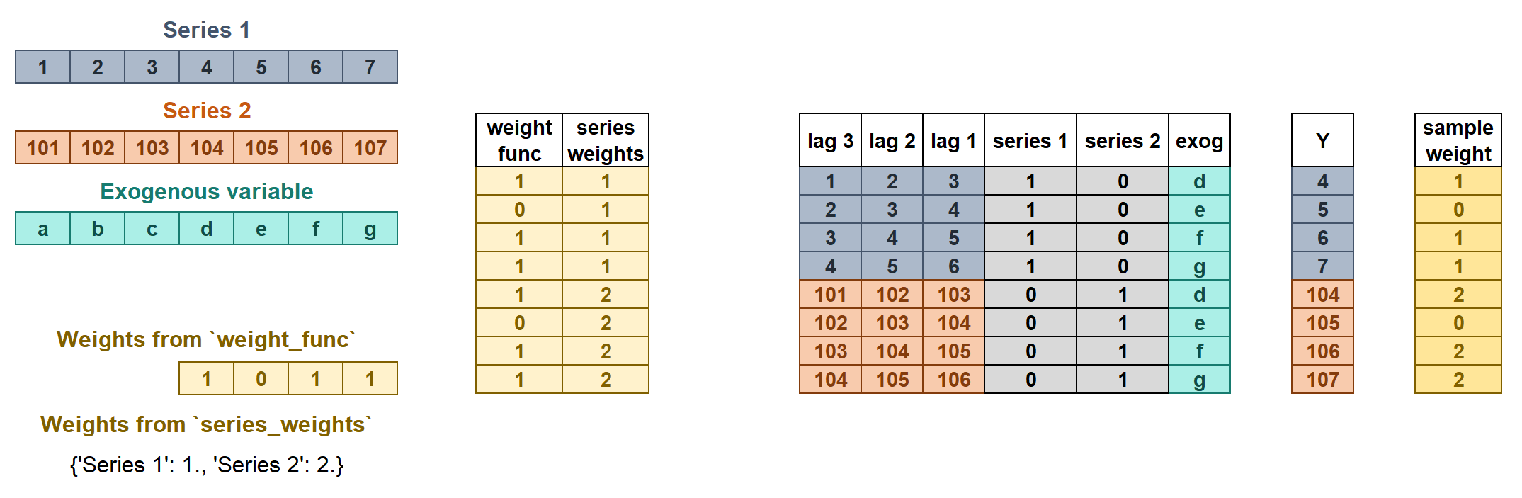
The weights are used to control the influence that each observation has on the training of the model. ForecasterRecursiveMultiseries accepts two types of weights:
series_weightscontrols the relative importance of each series. If a series has twice as much weight as the others, the observations of that series influence the training twice as much. The higher the weight of a series relative to the others, the more the model will focus on trying to learn that series.weight_funccontrols the relative importance of each observation according to its index value. For example, a function that assigns a lower weight to certain dates.
If the two types of weights are indicated, they are multiplied to create the final weights as shown in the figure. The resulting sample_weight cannot have negative values.
Learn more about weights in multi-series forecasting and weighted time series forecasting with skforecast.
In this example, item_1 has higher relative importance among series (it weighs 3 times more than the rest of the series), and observations between '2013-12-01' and '2014-01-31' are considered non-representative and a weight of 0 is applied to them.
# Weights in ForecasterRecursiveMultiSeries
# ======================================================================================
# Weights for each series
series_weights = {'item_1': 3.0} # Series not presented in the dict will have weight 1
# Weights for each index
def custom_weights(index):
"""
Return 0 if index is between '2013-12-01' and '2014-01-31', 1 otherwise.
"""
weights = np.where(
(index >= '2013-12-01') & (index <= '2014-01-31'),
0,
1
)
return weights
forecaster = ForecasterRecursiveMultiSeries(
estimator = HistGradientBoostingRegressor(random_state=123),
lags = 14,
transformer_series = StandardScaler(),
encoding = 'ordinal',
transformer_exog = None,
weight_func = custom_weights,
series_weights = series_weights
)
forecaster.fit(series=data)
forecaster.predict(steps=7).head(3)
╭────────────────────────────────── InputTypeWarning ──────────────────────────────────╮ │ Passing a DataFrame (either wide or long format) as `series` requires additional │ │ internal transformations, which can increase computational time. It is recommended │ │ to use a dictionary of pandas Series instead. For more details, see: │ │ https://skforecast.org/latest/user_guides/independent-multi-time-series-forecasting. │ │ html#input-data │ │ │ │ Category : skforecast.exceptions.InputTypeWarning │ │ Location : │ │ /home/ubuntu/anaconda3/envs/skforecast_22_py13/lib/python3.13/site-packages/skforeca │ │ st/utils/utils.py:2802 │ │ Suppress : warnings.simplefilter('ignore', category=InputTypeWarning) │ ╰──────────────────────────────────────────────────────────────────────────────────────╯
╭─────────────────────────────── IgnoredArgumentWarning ───────────────────────────────╮ │ {'item_50', 'item_33', 'item_21', 'item_35', 'item_49', 'item_3', 'item_48', │ │ 'item_4', 'item_2', 'item_19', 'item_36', 'item_47', 'item_26', 'item_18', │ │ 'item_42', 'item_39', 'item_29', 'item_14', 'item_11', 'item_15', 'item_25', │ │ 'item_43', 'item_30', 'item_12', 'item_23', 'item_6', 'item_45', 'item_38', │ │ 'item_10', 'item_40', 'item_9', 'item_34', 'item_44', 'item_5', 'item_41', │ │ 'item_16', 'item_24', 'item_32', 'item_28', 'item_13', 'item_46', 'item_17', │ │ 'item_22', 'item_31', 'item_20', 'item_7', 'item_27', 'item_8', 'item_37'} not │ │ present in `series_weights`. A weight of 1 is given to all their samples. │ │ │ │ Category : skforecast.exceptions.IgnoredArgumentWarning │ │ Location : │ │ /home/ubuntu/anaconda3/envs/skforecast_22_py13/lib/python3.13/site-packages/skforeca │ │ st/recursive/_forecaster_recursive_multiseries.py:1783 │ │ Suppress : warnings.simplefilter('ignore', category=IgnoredArgumentWarning) │ ╰──────────────────────────────────────────────────────────────────────────────────────╯
| level | pred | |
|---|---|---|
| 2018-01-01 | item_1 | 20.583876 |
| 2018-01-01 | item_10 | 61.580282 |
| 2018-01-01 | item_11 | 62.323468 |
✏️ Note
A dictionary can be passed to weight_func to apply different functions for each series. If a series is not presented in the dictionary, it will have weight 1.
Predict new series (unknown series)
ForecasterRecursiveMultiseries allows predicting unknown series (series not seen during the training process). Two scenarios may occur:
There is historical data for the new series: The user must provide a
DataFramewith the historical data required to create the features (lags and window features) used during the prediction process. ThisDataFramemust contain one column per series to be predicted. It is possible to include both series seen during training and new (unseen) series.There is no historical data for the new series: This scenario is similar, but the
last_windowfor the new series is composed entirely ofNaNvalues. This approach is only possible when using regressors that support missing values, since all lagged features will beNaN.
In both cases, exogenous variables may be available or not. If they are not available, they will be automatically set to NaN.
# Predict new series with available historical data
# ==============================================================================
# Create the last window with the last 14 observations of the new series
last_window_new = pd.DataFrame(
{
"series_new_1": [1671.50059509, 1544.75089264, 1478.75059509, 1336.50069427,
1277.75039673, 1003.25049591, 820.25009918, 1075.75049591,
1409.251091 , 1344.75059509, 1310.00039673, 1297.00089264,
1103.50039673, 871.50019836],
"series_new_2": [2695.2603035 , 1980.37118912, 1929.88060379, 1817.25070572,
1784.12020111, 1986.88029099, 2257.11999512, 2489.26069641,
1994.50059509, 1830.8717804 , 1776.25099182, 1644.001091,
1943.50058746, 3658.36999512]
},
index=pd.date_range("2016-07-18", periods=14, freq="D"),
)
forecaster.predict(steps=5, last_window=last_window_new)
╭──────────────────────────────── UnknownLevelWarning ─────────────────────────────────╮ │ `levels` {'series_new_2', 'series_new_1'} were not included in training. Unknown │ │ levels are encoded as NaN, which may cause the prediction to fail if the estimator │ │ does not accept NaN values. │ │ │ │ Category : skforecast.exceptions.UnknownLevelWarning │ │ Location : │ │ /home/ubuntu/anaconda3/envs/skforecast_22_py13/lib/python3.13/site-packages/skforeca │ │ st/utils/utils.py:1143 │ │ Suppress : warnings.simplefilter('ignore', category=UnknownLevelWarning) │ ╰──────────────────────────────────────────────────────────────────────────────────────╯
| level | pred | |
|---|---|---|
| 2016-08-01 | series_new_1 | 143.781101 |
| 2016-08-01 | series_new_2 | 143.781101 |
| 2016-08-02 | series_new_1 | 145.612148 |
| 2016-08-02 | series_new_2 | 145.612148 |
| 2016-08-03 | series_new_1 | 146.013700 |
| 2016-08-03 | series_new_2 | 146.013700 |
| 2016-08-04 | series_new_1 | 146.013700 |
| 2016-08-04 | series_new_2 | 146.013700 |
| 2016-08-05 | series_new_1 | 146.013700 |
| 2016-08-05 | series_new_2 | 146.013700 |
# Predict new series without available historical data
# ==============================================================================
# Create the last window with of the new series with nan values
last_window_new = pd.DataFrame(
{
"series_new_1": np.nan,
"series_new_2": np.nan
},
index=pd.date_range("2016-07-18", periods=14, freq="D"),
)
forecaster.predict(steps=5, last_window=last_window_new)
╭──────────────────────────────── UnknownLevelWarning ─────────────────────────────────╮ │ `levels` {'series_new_2', 'series_new_1'} were not included in training. Unknown │ │ levels are encoded as NaN, which may cause the prediction to fail if the estimator │ │ does not accept NaN values. │ │ │ │ Category : skforecast.exceptions.UnknownLevelWarning │ │ Location : │ │ /home/ubuntu/anaconda3/envs/skforecast_22_py13/lib/python3.13/site-packages/skforeca │ │ st/utils/utils.py:1143 │ │ Suppress : warnings.simplefilter('ignore', category=UnknownLevelWarning) │ ╰──────────────────────────────────────────────────────────────────────────────────────╯
╭──────────────────────────────── MissingValuesWarning ────────────────────────────────╮ │ `last_window` has missing values. Most of machine learning models do not allow │ │ missing values. Prediction method may fail. │ │ │ │ Category : skforecast.exceptions.MissingValuesWarning │ │ Location : │ │ /home/ubuntu/anaconda3/envs/skforecast_22_py13/lib/python3.13/site-packages/skforeca │ │ st/utils/utils.py:1223 │ │ Suppress : warnings.simplefilter('ignore', category=MissingValuesWarning) │ ╰──────────────────────────────────────────────────────────────────────────────────────╯
| level | pred | |
|---|---|---|
| 2016-08-01 | series_new_1 | 62.453964 |
| 2016-08-01 | series_new_2 | 62.453964 |
| 2016-08-02 | series_new_1 | 61.960619 |
| 2016-08-02 | series_new_2 | 61.960619 |
| 2016-08-03 | series_new_1 | 61.594364 |
| 2016-08-03 | series_new_2 | 61.594364 |
| 2016-08-04 | series_new_1 | 61.594364 |
| 2016-08-04 | series_new_2 | 61.594364 |
| 2016-08-05 | series_new_1 | 61.039157 |
| 2016-08-05 | series_new_2 | 61.039157 |
Conclusions
This use case shows that a multi-series model may have advantages over multiple individual models when forecasting time series that follow similar dynamics. Beyond the potential improvements in forecasting, it is also important to take into consideration the benefit of having only one model to maintain.
Session information
import session_info
session_info.show(html=False)
----- matplotlib 3.10.8 numpy 2.1.3 optuna 4.8.0 pandas 2.3.3 session_info v1.0.1 skforecast 0.22.0 sklearn 1.7.2 tqdm 4.67.3 ----- IPython 9.11.0 jupyter_client 8.8.0 jupyter_core 5.9.1 ----- Python 3.13.12 | packaged by Anaconda, Inc. | (main, Feb 24 2026, 16:13:31) [GCC 14.3.0] Linux-5.15.0-1084-aws-x86_64-with-glibc2.31 ----- Session information updated at 2026-04-23 13:01
Citation
How to cite this document
If you use this document or any part of it, please acknowledge the source, thank you!
Global Forecasting Models: Modeling Multiple Time Series with Machine Learning by Joaquín Amat Rodrigo and Javier Escobar Ortiz, available under a CC BY-NC-SA 4.0 at https://www.cienciadedatos.net/documentos/py44-multi-series-forecasting-skforecast.html
How to cite skforecast
If you use skforecast for a publication, we would appreciate it if you cite the published software.
Zenodo:
Amat Rodrigo, Joaquin, & Escobar Ortiz, Javier. (2024). skforecast (v0.22.0). Zenodo. https://doi.org/10.5281/zenodo.8382788
APA:
Amat Rodrigo, J., & Escobar Ortiz, J. (2024). skforecast (Version 0.22.0) [Computer software]. https://doi.org/10.5281/zenodo.8382788
BibTeX:
@software{skforecast, author = {Amat Rodrigo, Joaquin and Escobar Ortiz, Javier}, title = {skforecast}, version = {0.22.0}, month = {03}, year = {2026}, license = {BSD-3-Clause}, url = {https://skforecast.org/}, doi = {10.5281/zenodo.8382788} }
Did you like the article? Your support is important
Your contribution will help me to continue generating free educational content. Many thanks! 😊


This work by Joaquín Amat Rodrigo and Javier Escobar Ortiz is licensed under a Attribution-NonCommercial-ShareAlike 4.0 International.
Allowed:
-
Share: copy and redistribute the material in any medium or format.
-
Adapt: remix, transform, and build upon the material.
Under the following terms:
-
Attribution: You must give appropriate credit, provide a link to the license, and indicate if changes were made. You may do so in any reasonable manner, but not in any way that suggests the licensor endorses you or your use.
-
NonCommercial: You may not use the material for commercial purposes.
-
ShareAlike: If you remix, transform, or build upon the material, you must distribute your contributions under the same license as the original.